This paper presents a forecasting technique for forward energy prices, one day ahead. This technique combines a wavelet transform and forecasting models ...
Combining the Wavelet Transform and Forecasting Models to Predict Gas Forward Prices Hang T. Nguyen, Ian T. Nabney Neural Computing Research Group School of Engineering and Applied Science Aston University, United Kingdom {thihangn, i.t.nabney}@aston.ac.uk Abstract This paper presents a forecasting technique for forward energy prices, one day ahead. This technique combines a wavelet transform and forecasting models such as multilayer perceptron, linear regression or GARCH. These techniques are applied to real data from the UK gas markets to evaluate their performance. The results show that the forecasting accuracy is improved signi cantly by using the wavelet transform. The methodology can be also applied to forecasting market clearing prices and electricity/gas loads.
1. Introduction Accurate electricity/gas price forecasting is very important for traders in the energy market, especially energy generators. If an energy generator makes an accurate forecast of the market price, it can develop a strategy to maximise its own pro ts and minimise risk due to price spikes by appropriate trading in forward contracts. It can also plan its actions to maximise bene ts or utilities by reducing/increasing its generation. Energy suppliers can use short-term price forecasts to adjust their bidding strategies to achieve the maximum bene t. In addition, understanding the process of forward price development can help the generators make money on the forward market. A number of statistical methodologies have been proposed for energy price forecasting. Many approaches based on time series models have been used for price forecasting, such as threshold auto-regressive switching (TAR) models [1], AR models [2], autoregressive integrated moving average (ARIMA) models [3], [4], and generalised autoregressive conditional heteroschedasticity (GARCH) [5], [6]. Moreover, neural networks (NNs) are used widely for electricity price forecasting in the literature [7]. Due to the
complexity of the environment, the functional relationships we are looking for might be non-linear. Several researchers have proposed additional procedures to improve accuracy. Pre-processing procedures and regularisation methods are used in [7]. Another approach for improving forecasting performance is multiple NNs. The use of a committee of NNs for forecasting is suggested in [8]. Similarly, cascaded neural networks are proposed in [9]. The use of Input/Output Hidden Markov Model (IOHMM) to combine two NNs which estimate underlying market states and observed price respectively are suggested in [10]. However, forecasting energy prices presents a number of challenges because of the volatility characteristic of prices, especially in such a competitive environment [5]. To overcome this problem, multiresolution decomposition techniques such as the wavelet transform (WT) have been used as a pre-processing procedure. The WT can produce a good local representation of the signal in both the time and frequency domain. Daubechies WT was combined with a forecasting model to forecast spot electricity prices and electricity load in [4], [11], [12], [13]. Because this type of wavelet is symmetric, the wavelet coef cients takes into account future information. However, when forecasting, we can only use data obtained earlier in the time domain. So, symmetric WTs, such as Daubechies or Morlet, are not suitable for this type of application. Several papers have mentioned this problem and use an à trous wavelet transform or a redundant Haar wavelet transform in nancial time series forecasting [14], and electricity load forecasting [15], [16], [17]. This paper uses a combination of the redundant Haar wavelet transform (RHWT) and prediction models to forecast gas prices of forward contracts. We compare the prediction performance of four methods: Method 1: a random walk model, which is used as a benchmark. Method 2: prediction models without WT. The predic-
tion models include linear regression (LR), Multi-layer Perceptron (MLP), and GARCH. Method 3: a combination of RHWT and a forecast model where each component of WT is separately forecasted (multicomponent forecast). Method 4: using the components of RHWT as input variables for a forecast model to directly predict the original price (direct forecast). Compared with previous work, our paper makes the following contributions. Firstly, we compared the prediction accuracy of using WT in two approaches: (1) separately forecasting each WT components and combining the predictions and (2) directly forecasting original price. Secondly, besides historical price data and its WT components, a number of exogenous variables, for example, gas demand, temperature, exchange rate (USD:GBP) etc, are also considered as candidates for input variables. Some preprocessing procedures are used to choose the relevant input variables for each forecasting model. Thirdly, we tried to combine the WT with different forecasting methods (MLP, LR, and GARCH). The experiment results show that multicomponent forecast with GARCH are better than the others. Fourthly, while existing papers applied WT for predicting electricity load, electricity spot price or exchange rate, we tried to use it forecasting for price of forward contracts in the gas market. Fifthly, we analysed the correlation of residuals of components when using multicomponent forecast and have shown the residuals of WT components are highly correlated. This paper is organised as follows. Section 2 provides the detailed forecasting framework. In Section 3, the RHWT for decomposing data into components is presented. The GARCH, MLP and LR forecasting models are described in Section 4. Numerical results on data from the UK gas market are given in Section 5. Section 6 provides some conclusions.
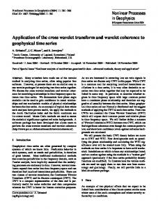
2. Forecasting Framework The framework of Method 3 for forecasting is shown in Figure 1. This is a combination of forecasting models and the RHWT. A data set is divided into two sub-data sets: (1) a training set to estimate the model parameters and (2) a test set to evaluate these models by calculating appropriate error functions. It is summarised in four steps as follows: Step 1: Use the RHWT to decompose the real price of gas of the training set and the test set separately: A; Dn ; Dn 1 ; :::; D1 . Each component represents the data in a frequency range that is less volatile and easier to forecast than the original time series.
Figure 1. The combination of RHWT and prediction models (Method 3). (a) Training phase, (b) Test phase.
Step 2: Determine the input vectors for each model for predicting each component. In addition to the historical price data, there is a large number of observable variables which are potential inputs. However, only some of them are relevant. Using irrelevant variables as inputs might reduce the performance of the forecasting models. Therefore, selecting correct inputs for each type of model is very important. In the training phase, various measures were used to determine the relevant input variables, including the correlation matrix (CM), autocorrelation function (ACF), and partial autocorrelation function (PACF). Step 3: The training sets are used to develop forecasting models (i.e. estimate parameters), one forecasting model for each component. In the test phase, the developed models (i.e. with the determined parameters) are used to predict the future value of the components from the current observable data. The outputs of these models at time t are the values of A; Dn ; Dn 1 ; :::; D1 at time step t + 1. In this work, three models were used for forecasting: LR, MLP, and GARCH. Step 4: In the test phase, the inverse WT is used to compute the price from the predictions of components.
3. Redundant Haar wavelet transform 3.1. Why RHWT? In several popular WTs, such as Daubechies or Symlets, there can be problems with signal boundaries: if we add or delete the last few data points of a time series, the wavelet coef cients will change at some boundary time points [15]. The reason is that these WTs are symmetric wavelets, which
before time step 2i+1 1. After applying the redundant Haar wavelet transform, this paper will consider only those coef cients after time step 2n 1. In this paper, we ran experiments with several decomposition levels. The most accurate forecasting were with 2-level WT, and these results will are reported in Section 5. An example of decomposing by redundant Haar wavelet transform is shown in Figure 3.This data shows the price of a monthly forward product in the UK gas market. Comparing to the original data, the approximation coef cient A is much smoother, and the detail coef cients D2 and D1 are less volatile and contain periodic elements. Therefore, they are easier to forecast than the original price.
4. Forecasting models 4.1. Linear regression Figure 2. Computation of wavelet coef cients of different scales in the RHWT.
take into account future values when computing coef cients of a time series. Therefore, we cannot use these symmetric WTs for forecasting applications. The Haar WT is asymmetric and can be used in prediction. Normally, a discrete wavelet transform has two stages: (1) computing detail and approximation coef cients with high- and low-pass lters, and (2) decimation, i.e. retaining one sample out of every two. The main advantage of decimation is reducing the storage requirement. However, decimation leads to the loss of phase information. To overcome this, we can use a redundant or non-decimated wavelet transform [15]. In a redundant WT, only stage (1) is completed. All components of a redundant WT have the same length as the original time series. Therefore, there is a one-to-one correspondence between the original data and decomposition coef cients at a given time step.
3.2. Computing the RHWT Assuming that there is a time series p(t), t = 1; 2; :::; T , Figure 2 shows how to compute its redundant Haar wavelet transform coef cients to the n-th decomposition level. At level i, the detail coef cients Di are retained, while the approximation coef cients Ai are decomposed into a further level of detail Di+1 and approximation coef cient Ai+1 . It can be shown that the original time series can now be reconstructed as: p(t) = An (t) + Dn (t) + + D1 (t). Note that to calculate a coef cient at level i + 1 at time t (Ai+1 (t) or Di+1 (t)), we need to use the value of time series Ai at time step t 2i . Therefore, at level i + 1, it is impossible to exactly de ne the value of these coef cients
Linear regression is a simple model where the output is linear combination of inputs. Unlike the AR, ARMA, or ARIMA models, the input vector of a linear regression can include both historical values of target variables and exogenous variables (e.g. exchange rate, other components of RHWT, etc.). This model is given by: y=
d X
wi xi = wT x,
i=0
where y represents the output of target data, w is the weight vector (w0 ; w1 ; :::; wd ), w0 is called bias of the model, and x represents the input vector x = (x0 ; x1 ; :::; xd ), x0 = 1 for the bias. Detail explanation of training this model is given in [18]
4.2. Multi-layer perceptron A multi-layer perceptron consists of a number of perceptrons organized by layers. Each perceptron has several inputs and one output, which is a non-linear function of the inputs. It has been shown that networks with just two layers (i.e. inputs, hidden units, and output layer) are capable of approximating any continuous functional mapping if the number of hidden units is large enough [19]. Therefore, only two-layer networks will be considered. During training an MLP model, we often encounter overtting. Over tting is a problem where the model ts the noise in the training data rather than the underlying generator, and may lead to large errors on unseen data. There are several approaches to overcome this problem, such as early stopping or using a committee to combine different networks. In this paper, we use weight decay to regularise the model by penalising large weights and imposing smoothness. The Bayesian evidence procedure is used to compute the optimal hyper-parameters [20].
zero-mean noise. The model predicts that the next value of the time series is the same as the current value.
4.5. Model evaluation To evaluate the prediction performance of these models, four types of prediction errors of the test sets were computed. They are the mean absolute percentage error (MAPE), mean squared error (MSE), root mean squared error (RMSE), and mean absolute error (MAE), which are dened by eM AP E Figure 3. An example of RHWT with decomposition level 2. (a) price data, (b) approximation coef cient A, (c) detail coef cient D2 , (d) D1
eM SE eRM SE eM AE
The number of hidden units is set to be the average of the number of inputs and the number of outputs [14].
4.3. GARCH So far, the errors are assumed to be homoschedastic (i.e., the variance of the residual is assumed to be independent of time). GARCH can be used to model changes in the variance of the errors as a function of time. GARCH was rstly proposed by Bollerslev (1986) and is frequently used in nancial forecasting. The GARCH(r; m) model is given by: yt ht
1 XT yreal yf orecast 100% 1 T yreal PT 2 yf orecast ) 1 (yreal = PT 2 y) 1 (yreal p = eM SE 1 XT jyreal yf orecast j , = 1 T =
where yreal is the real gas price, yf orecast is the forecast gas price, y is the mean of yreal , and T is the number of data points. We also computed the improvement ratio (IR) of errors of a method comparing to errors of the RW model. Errors here may be MAPE, MSE, RMSE or MAE. For example, the IR of MSE of a model M comparing to MSE of the RW is given by: IRM SE (M )=
eM SE (RW ) eM SE (M ) 100%. eM SE (RW )
5. Experimental results
0
= xt + "t ; Pm = 0+ i=1
"t D(0; ht ) Pr 2 i "t i + j=1 j ht j Pm Pr with constraints: i ; j > 0; i=1 i + j=1 j < 1, where xt , yt , and "t represent the input vector, output vector, and error of the model respectively, ht is variance of error "t , is the parameter vector for the AR process, m and r are order of ARCH process and AR for the variance h respectively. "t is i.i.d, with E("t ) = 0 and var("t ) = ht . "t can be a Gaussian or Student-t distribution. GARCH is a generalisation of a linear time series model with homoschedastic disturbances in which the conditional mean ht of the noise varies with information about errors and its variance up to time t.
4.4. Random walk The random walk (RW) is used as a benchmark model. This model is given by: y(t + 1) = y(t) + "(t), where " is a
The data used in this work is taken from the UK gas market, provided by E.ON UK plc. This company is interested in the daily price of monthly gas products. The monthly gas product is a forward contract for supplying gas in a single month in the future. In the UK gas market, it is possible to trade gas from one to six month(s) ahead. For each monthly product (e.g. July 2006) there is approximately 6 months of daily price data (approximately 130 data points). For example, the July 2006 product can be traded from 03 Jan 2006 to 30 Jun 2006. To illustrate the behaviour of the proposed methods, six data sets are used (shown in Figure 4). The test sets of the rst three data sets correspond to the beginning, middle and end of a stable monthly product. The test sets of the last three data sets correspond to the beginning, middle and end of a volatile monthly product. If a test set of a data set is the beginning or middle of a monthly gas product trading period, the training set are data of another monthly product. For example, in data set 2 (Figure 4 (b)), the test set is the middle samples of March 2007 product
Figure 4. Six data sets used in the experiments (a-f). The thin lines are the training sets and the bold lines are the test sets.
and the training set is November 2006 product. The prices for different products are different even in the same trading day; for example, the price of a colder month is normally higher than that of a warmer month. This is the reason why there is gap between the training sets and test sets of these data sets in Figure 4. The average errors of each method for the six data sets are presented in Table 1. We compared the prediction performance of the proposed method (Method 3 in Section I) with a random walk model (Method 1) and two other approaches (Method 2, 4) which are shown in Figure 5. Like Method 3, the real price time series in the Method 4 is also decomposed into components. These components and exogenous variables are also used as candidates for input variables. However, the main difference between Method 4 and Method 3 is that Method 4 directly forecasts the price while Method 3 separately forecasts wavelet transform components and the predicted price is derived from these forecast components by using the inverse wavelet transform. Therefore, Method 4 has only one forecast model while Method 3 has several forecast models, one model for each coef cient. In all methods, the training sets are used to compute the parameters of the model. Then these developed models are used to compute the future values of the test set. The errors of the test set are calculated to evaluate prediction performance. Table 1 provides the average IRM SE , MSE, MAPE, MAE, and RMSE for the six data sets of the methods.
Figure 5. Two methods for forecasting gas price. (a) Method 4, (b) Method 2.
For the purpose of comparison, these errors are computed for four methods as mentioned in Section I. "LR", "LR+RHWT3", "LR+RHWT4" refer to Method 2, 3, and 4 respectively with forecast model LR. The similar notations are used for MLP and GARCH models. "Method 1(RW)" refers to Method 1. "Method 2" is average error of different model (LR, MLP, GARCH) using Method 2. The similar notations are used for Method 3 and 4. The multicomponent forecast (Method 3) outperforms the others. The GARCH+RHWT3 is the best with MSE of 0.09485, its MSE improves 20% compared to the MSE of the random walk model. Method 3 is signi cantly better than Method 2, which proves the usefulness of the wavelet transform. The multicomponent forecast achieves better results than the direct forecast (Method 4). Table 2 shows the average MSE of forecasting individual components in LR+RHWT3, MLP+RHWT3, and GARCH+RHWT3 for six data sets. The average improvement ratio of MSEs of these models compared to the MSE of the RW are shown in Table 3. The errors on each component of these models are much smaller than random walk model. However, the sum of all the components (i.e. the price) of these models are not much better than the error of the random walk model. For example, the MSEs of the components A, D2, D1 in the GARCH+RHWT3 improved 85.39%, 77.77%, and 39.95% respectively, compared to these in the random walk model while the improvement ratio for the sum of all components (i.e. price) is only 20.05%. To investigate the relatively small improvement of the overall performance, we analysed the correlation matrix of residuals of components in the method GARCH+RHWT3 (see Table 4). The component residuals are quite highly
Table 4. The correlation matrix of residuals of components in the method GARCH+RHWT3.
Table 1. Average errors for the six data sets of methods.
Table 2. MSE of individual components and original price using different prediction models.
Figure 6. Residuals of components A (a), D2 (b), and D1 (c) using GARCH+RHWT3 for the test set 2.
correlated, especially components D1 and D2. Their correlation coef cient is 0.96144. Figure 6 shows the residuals of the test set 2 using GARCH+RHWT3. The residual of a component is the difference between the and the predicted value and real value of that component. The shape of the residuals of components D1 and D2 are similar. The residuals of these components are normally the same sign, so their sum has a large magnitude. In the RW model, the signs of component residuals are normally different, so they cancel when they are summed up. This is the reason why the prediction performance of total of components in GARCH+RHWT3 are not much better than the RW model, even though the accuracy of each component is much better than RW model.
6. Conclusions
Table 3. Improvement ratio of MSE of method 3 comparing to MSE of the RW model.
The results show that the use of wavelet transform as a pre-processing procedure of forecasting data improves the performance of prediction techniques. The multicomponent forecasting outperforms the methods without wavelet transform or direct forecasting. The results show that the residuals of components D1 and D2 are highly correlated. We will further investigate this issue and how to use this property to improve the results of the forecasting techniques. This paper forecasts daily gas prices for the monthly for-
ward product as an example to verify the performance of the proposed method. It can be used for other types of forward gas products, forward electricity products, and electricity/gas demand forecasts. Our proposed methods can be used to forecast more than one step ahead by replacing the single-output forecasting models by multi-output forecasting models (excepting the GARCH model).
7. Acknowledgment Hang T. Nguyen would like to thank to E.ON UK plc. for their nancial support. The authors are grateful to Matthew Cullen, Stuart Grif ths, Nick Sillito, Daniel Crispin and David Jones from E.ON for providing the data sets, and their valuable advice. Some parts of program have been written using the source code from the N ETLAB toolbox by Ian Nabney (available at http://www.ncrg.aston.ac.uk/netlab/).
References [1] M. Stevenson, “Filtering and forecasting spot electricity price in the increasingly deregulated australian electricity market”, in The International Institute of Forecaster Conference, Atlanta, 2001. [2] F.J. Nogales, J. Contreras, A.J. Conejo, and R. Espinola, “Forecasting next-day electricity prices by time series models”, IEEE transaction on Power system, vol. 17, no. 2, pp. 342–348, 2002. [3] J. Contreras, R. Espinola, F.J Nogales, and A.J. Conejo, “Arima models to predict next-day electricity prices”, IEEE transactions on Power Systems, vol. 18, no. 3, pp. 1014–1020, 2003. [4] Antonio J. Conejo, Miguel A. Plazas, Rosa Espinola, and Ana B. Molina, “Day-ahead electricity price forecasting using the wavelet transform and arima models”, in IEEE Transactions on Power Systems, 2005, vol. 20, pp. 1035–1042. [5] Z. Hua, X. Li, and L. Z. Zhang, “Electricity price forecasting based on garch model in deregulated market”, in Power Engineering Conference, USA, 2005. [6] R. C. Garcia, J. Contreras, M. V. Akkeren, and J. B. C. Garcia, “A garch forecasting model to predict dayahead electricity prices”, in IEEE Transactions on Power Systems, 2005, vol. 2, pp. 867– 874. [7] F. Gao, X. Guan, X.R. Cao, and A. Papalexopoulos, “Forecasting power market clearing price and quantity using neural network method”, in Proc. Power Engineering Summer Meet, Seattle, 2000, vol. 4, pp. 2183–2188.
[8] J. J. Guo and P. B. Luh, “Improving market clearing price prediction by using a committee machine of neural networks”, IEEE Transactions on Power Systems, vol. 19, no. 4, pp. 1867–1876, 2004. [9] L. Zhang, P.B. Luh, and K. Kasiviswanathan, “Energy clearing price prediction and con dence interval estimation with cascaded neural networks”, in IEEE Transaction on Power System, 2003, vol. 1, pp. 99– 105. [10] A. M. Gonzalez, A. M. S. Roque, and J. GarciaGonzalez, “Modeling and forecasting electricity prices with input/output hidden markov models”, IEEE Transactions on Power Systems, vol. 20, no. 1, pp. 13–24, 2005. [11] T. Nengling, J. Stenzel, and W. Hongxiao, “Techniques of applying wavelet transform into combined model for short term load forecasting”, Electric Power Systems Research, vol. 76, pp. 525–533, 2005. [12] C. Kim, I. K. Yu, and Y. H. Song, “Kohonen neural network and wavelet transform based approach to short-term load forecasting”, Electronic Power System Research, vol. 63, pp. 169–176, 2002. [13] H. Xu and T. Niimura, “Short-term electricity price modeling and forecasting using wavelets and multivariable time series”, in Power Systems Conference and Exposition, 2004. [14] B. L. Zhang, R. Coggins, D. Dersch, and B. Flower, “Multiresolution forecasting for futures trading using wavelet decompositions”, IEEE Transactions on Neural Networks, vol. 12, no. 4, 2001. [15] J. L. Starck and F. Murtagh, “Mr/ nance multiresolution analysis of time series”, Online, 2001. [16] D. Benaouda, F. Murtagh, J. L. Starck, and O. Renaud, “Wavelet-based nonlinear multiscale decomposition model for electricity load forecasting”, Neurocomputing, vol. 70, pp. 139–154, 2006. [17] Z. Y. Dong, B. L. Zhang, and Q. Huang, “Adaptive neural network short term load forecasting with wavelet decomposition”, in IEEE Porto Power Tech Conference, 2001. [18] I. T. Nabney, NETLAB: Algorithms for Pattern Recognition, Great Britain: Springer, 2002. [19] K. Hornik, M. Stinchcombe, and H. White, “Multilayer feedforward networks are universal approximators”, Neural Networks, vol. 2, no. 5, pp. 359–366, 1989. [20] D. J. C. Mackay, “Bayesian interpolation”, Neural Computation, vol. 4, pp. 415–447, 1992.