Short-Term Load Forecasting Based on Wavelet Transform and Least ...

Hindawi Publishing Corporation Journal of Electrical and Computer Engineering Volume 2015, Article ID 862185, 9 pages http://dx.doi.org/10.1155/2015/862185

Research Article Short-Term Load Forecasting Based on Wavelet Transform and Least Squares Support Vector Machine Optimized by Fruit Fly Optimization Algorithm Wei Sun and Minquan Ye Department of Business Administration, North China Electric Power University, Baoding 071000, China Correspondence should be addressed to Minquan Ye; [email protected] Received 6 October 2015; Revised 17 November 2015; Accepted 29 November 2015 Academic Editor: George S. Tombras Copyright © 2015 W. Sun and M. Ye. This is an open access article distributed under the Creative Commons Attribution License, which permits unrestricted use, distribution, and reproduction in any medium, provided the original work is properly cited. Electric power is a kind of unstorable energy concerning the national welfare and the people’s livelihood, the stability of which is attracting more and more attention. Because the short-term power load is always interfered by various external factors with the characteristics like high volatility and instability, a single model is not suitable for short-term load forecasting due to low accuracy. In order to solve this problem, this paper proposes a new model based on wavelet transform and the least squares support vector machine (LSSVM) which is optimized by fruit fly algorithm (FOA) for short-term load forecasting. Wavelet transform is used to remove error points and enhance the stability of the data. Fruit fly algorithm is applied to optimize the parameters of LSSVM, avoiding the randomness and inaccuracy to parameters setting. The result of implementation of short-term load forecasting demonstrates that the hybrid model can be used in the short-term forecasting of the power system.

1. Introduction Power load forecasting is an important part of management modernization of electric power systems, which has attracted more and more attentions from the academic circle and the practice. Power load forecast with high precision can ease the contradiction between power supply and demand, providing a solid foundation for the stability and reliability of the power grid. It can avoid the waste of resources in the process of grid scheduling and improve the economic benefit. Thus, improving load forecasting methods and the accuracy of prediction constantly is of great important significance to formulate the economic and better power generation plan, reduce spinning reserve capacity, analyse power market demand, and so forth. However, the power load will be influenced by many factors, so features like irregularity and linear independence do exist, which result in the difficulty in making accurate predictions to the power load. At present, the methods for load forecasting can be divided into two parts: classical mathematical statistical methods and approaches based on artificial intelligence. Most load forecasting theories are based on time series analysis

and autoregression models, including vector autoregression model (VAR) and autoregressive moving average model (ARMA) [1–5]. Time series smoothness prediction methods are criticized by researchers for their weakness of nonlinear fitting capability. With the development of the electricity market, the requirement of high accuracy load forecasting is more strict and efficient. So artificial intelligence, which includes neural network [6–8], grey model [9, 10], and support vector machine [11], gains more and more attention from scholars. Due to the strong self-learning, self-adapting ability, and nonlinear change character, artificial neural network is widely used in prediction field. Kandil et al. [12] applied artificial neural network (ANN) for short-term load forecasting without the use of load history and only temperature was used, and it was proved to be effective. After that, BPNN [13] and GRNN [14] are used in improving ANN model for excellent predictive abilities. The shortcomings of neural networks are the requirement of a large amount of data, a long time solving which may cause easily falling into local optimum. Support vector machine (SVM) is a new statistical learning method [15]. Compared with other machine learning methods, SVM implement the structural risk minimization

2 principle to minimize an upper bound on the generalization error, rather than employing the empirical risk minimization principle to minimize the training error, and it gives SVMs better generative performance. As an extension of SVM, least squares support vector machine (LSSVM) transforms the second optimal inequality constraints problem in original space into equality constraints’ linear system in feature space through nonlinear mapping [16], which improved the speed and accuracy of convergence. Different parameters selection in LSSVM (Kernel parameter and penalty factor) would have big influences on the fitting accuracy and generalization ability; inappropriate parameter selection may lead to the limitation of the performance of LSSVM. However, it is possible to employ an optimization algorithm to obtain an appropriate parameter combination. Particle swarm optimization model [17], genetic algorithm model [18], and Firefly Algorithm [19] model are all proposed in parameter optimization for LSSVM; for example, particle swarm optimization finds overall optimal value by following the currently found optimal values. But premature convergence and easily falling into local optimum restrict the application of the particle swarm optimization. Thus, this paper puts forward fruit fly optimization model to optimize the parameters of LSSVM. Fruit fly optimization algorithm was proposed by Pro. Pan [20] in Taiwan in 2012. The FOA has the advantages of being easy to understand due to the shorter program code compared with other optimization algorithms and reaching a better global optimal solution. Li et al. [21] applied the FOA to optimize the parameters of GRNN in order to forecast the annual power load. Zheng et al. [22] proposed a novel fruit fly algorithm for the semiconductor final testing scheduling problem. Pan et al. [23] developed an improved FOA algorithm for continuous function optimization problems. The wavelet transform (WT) is a recently developed mathematical tool for signal analysis. It has been applied successfully in astronomy, data compression, signal and image processing, earthquake prediction, and so on [12]. The combination of WT and LSSVM is widely used in forecasting fields [24, 25]. This paper proposes WT to reprocess the data and improve its reliability. In order to enhance the accuracy of load forecasting, WT-FOA-LSSVM is put up with, and the examples demonstrate the effectiveness of the model. The rest of the paper is organized as follows: Section 2 provides some basic theoretical aspects of WT, LSSVM, and FOA and gives a brief description about WT-FOA-LSSVM model; in Section 3, an experiment study is put forward to prove the efficiency of the proposed model; Section 4 is the conclusion of this paper.

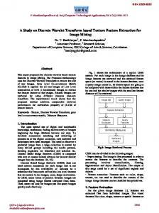
2. WT-FOA-LSSVM Model 2.1. Wavelet Transform. Wavelet transform is a mathematical tool for signal analysis which developed in recent decades. It can capture the frequency and location information of the input signal. The basic concept in wavelet transform is to decompose a signal into an approximation component and detail components, in which approximation component is the low-frequency information and contains the important information of the signal. The details are the high-frequency

Journal of Electrical and Computer Engineering

S

A1

A2

D1

D2

Figure 1: Wavelet decomposition.

components which are related to the small-scale space in the signal. Figure 1 is a wavelet decomposition tree showing the decomposition process. In order to overcome the high redundancy situation which exists in continuous wavelet transform, it captures both frequency and location information in temporal resolution. We propose the discrete wavelet transform (DWT) in this paper, and it is defined as follows: 𝜓𝑎,𝑏 (𝑡) = 𝜓1/2𝑗 ,𝑘/2𝑗 (𝑡) = 2𝑗/2 𝜓 (2𝑗 𝑡 − 𝑘) ,

(1)

where the scale factor 𝑎 = 1/2𝑗 , 𝑗 ∈ 𝑍, and the displacement factor 𝑏 = 𝑘/2𝑗 , 𝑗 ∈ 𝑍. In general, 𝜓𝑗,𝑘 (𝑡) represents the discrete transform. Using DWT in the signal 𝑓(𝑥), the formula can be shown as (𝑊𝜓 𝑓) (𝑗, 𝑘) = ⟨𝑓, 𝜓𝑗,𝑘 (𝑡)⟩ = ∫

+∞

−∞

𝑓 (𝑡) 𝜓𝑗,𝑘 (𝑡) 𝑑𝑡.

(2)

In this paper, the original load signal is proposed to be decomposed into an approximation component and some detail components. The approximation presents the main fluctuation of the load and the details to contain the spikes and stochastic volatilities. A suitable number of levels can be decided by comparing the similarity between the approximation and the original signal. 2.2. Least Squares Support Vector Machine. LSSVM is an extension of the standard support vector machine (SVM), proposed by Suykens and Vandewalle [26]. It transforms the inequality constraints of traditional SVM into equality constraints and considers sum squares error loss function as the loss experience of the training set, which transforms solving quadratic programming problems into solving linear equations problems [27]. The training set is set as {(𝑥𝑘 , 𝑦𝑘 ) | 𝑘 = 1, 2, . . . , 𝑛}, in which 𝑥𝑘 ∈ 𝑅𝑛 is the input data and 𝑦𝑘 ∈ 𝑅𝑛 is the output data. 𝜑(⋅) is the nonlinear mapping function which transfers the samples into a much higher dimensional feature space 𝜙(𝑥𝑘 ). Establish the optimal decision function in the high-dimensional feature space: 𝑦 (𝑥) = 𝜔𝑇 ⋅ 𝜑 (𝑥) + 𝑏,

(3)

where 𝜑(𝑥) is mapping function; 𝜔 is weight vector; 𝑏 is constant.

Journal of Electrical and Computer Engineering

3

Using the principle of structural risk minimization, the objective optimization function is as follows: 1 𝑛 1 min (𝜔, 𝑒) = 𝜔𝑇 𝜔 + 𝛾 ∑ 𝑒𝑘2 . 𝜔,𝑏,𝑒 2 2 𝑘=1

(4)

Its constraint condition is 𝑦𝑘 = 𝜔𝑇 𝜑 (𝑥𝑘 ) + 𝑏 + 𝑒𝑘 , 𝑘 = 1, 2, . . . , 𝑛,

𝐿 (𝜔, 𝑏, 𝑒, 𝛼) = 𝜙 (𝜔, 𝑒) − ∑ {𝛼𝑘 [𝜔𝑇 𝜑 (𝑥𝑘 ) + 𝑏 + 𝑒𝑘 − 𝑦𝑘 ]} ,

Interactive evolution Fruit fly 2 (X2 , Y2 )

Fruit fly 3 (X3 , Y3 )

(5)

in which 𝛾 is the penalty coefficient and 𝑒𝑘 is slack variable. Define the Lagrange function to solve the problem: 𝑛

Food

Dist2

Fruit fly group (X, Y)

Dist3 Fruit fly 1 (X1 , Y1 )

(6) Dist1

𝑘=1

where Lagrange multiplier 𝛼𝑘 ∈ R. According to the Karush-Kuhn-Tucker (KKT) conditions, 𝜔, 𝑏, 𝑒𝑘 , 𝛼𝑘 are taken as partial derivatives and required as zero. Consider 𝑛

𝜔 = ∑ 𝛼𝑘 𝜑 (𝑥𝑘 ) , 𝑘=1

𝑛

∑ 𝛼𝑘 = 0,

𝑘=1

(7)

𝛼𝑘 = 𝑒𝑘 𝛾, 𝜔𝑇 𝜑 (𝑥𝑘 ) + 𝑏 + 𝑒𝑘 − 𝑦𝑘 = 0. According to (7), the optimization problem can be transformed into solving linear problem, which is shown as follows: 0 1 ⋅⋅⋅ 1 𝑏 ] [ 1 ] [𝛼 ] [1 𝐾 (𝑥1 , 𝑥1 ) + , 𝑥 ) ⋅ ⋅ ⋅ 𝐾 (𝑥 1 𝑙 ] [ 1] [ 𝛾 ][ ] [ ][ . ] [ .. .. .. .. ][ . ] [. . . . ][ . ] [ [ 1] 1 𝐾 (𝑥𝑙 , 𝑥1 ) ⋅ ⋅ ⋅ 𝐾 (𝑥𝑙 , 𝑥𝑙 ) + [𝛼 ] 𝛾] 𝑙 [ (8) 0 [ ] [𝑦1 ] [ ] = [ . ]. [ .. ] [ ] [ 𝑦𝑙 ] Solve formula (8) to get 𝛼 and 𝑏; then the LSSVM optimal linear regression function is 𝑙

𝑓 (𝑥) = ∑ 𝛼𝑘 𝐾 (𝑥, 𝑥𝑘 ) + 𝑏.

(9)

𝑘=1

According to Mercer condition, 𝐾(𝑥, 𝑥𝑖 ) = 𝜑(𝑥)𝑇 ⋅𝜑(𝑥𝑙 ) is kernel function. In this paper, set radial basis function (RBF) as kernel function which is shown in the following equation: 󵄨2 󵄨󵄨 󵄨𝑥 − 𝑥𝑘 󵄨󵄨󵄨 (10) ), 𝐾 (𝑥, 𝑥𝑘 ) = exp (− 󵄨 2𝜎2 2

where 𝜎 is the width of kernel function.

Figure 2: Food finding iterative process of a fruit fly swarm.

From the problems of training LSSVM, kernel parameter 𝜎2 and penalty parameter 𝛾 are generally set based on experience, which leads to the existence of randomness and inaccuracy in the application of the LSSVM algorithm. To solve the problem, the paper uses fruit fly optimization algorithm to optimize these two parameters to improve the prediction accuracy of LSSVM. 2.3. Fruit Fly Optimization Algorithm. Fruit fly optimization algorithm is a kind of intelligent optimization algorithms based on fruit fly foraging behaviours proposed by Pan [20] in 2012. The basic concept of FOA is that fruit fly perceives food concentration according to its position, and then it will move to the site of maximum or minimum concentration by comparing flavor concentration; finally the objective function extreme value can be obtained through repeated iterations of food concentration. Food finding iterative process of fruit fly swarm is shown in Figure 2. According to the food finding characteristics of fruit fly swarm, the fruit fly optimization algorithm can be divided into following steps: (1) Randomly initialize the fruit fly swarm location (𝑥 axis, 𝑦 axis). (2) Give the random flight direction and the distance for food finding of an individual fruit fly by using olfactory: 𝑋𝑖 = 𝑥 axis + Random Value 𝑌𝑖 = 𝑦 axis + Random Value.

(11)

(3) Calculate the distance between the origin and each individual fruit fly position (Dist), and then calculate the value of flavor concentration (𝑆); it is the reciprocal of distance: Dist = √𝑋𝑖2 + 𝑌𝑖2 𝑆=

1 . Dist

(12) (13)

4

Journal of Electrical and Computer Engineering

(4) Put the value of flavor concentration 𝑆 into its fitness function, and then get the flavor concentration of the individual fruit fly location (Smell). (5) Find out the individual fruit fly with minimal smell concentration among the fruit fly swarm: [best Smell, best index] = max (Smell) .

(14)

(6) Retain the best flavor concentration and its 𝑋, 𝑌 coordinates, and then the fruit flies fly to the position by using vision. Enter iterative optimization to repeat steps (2)–(5). When the fitness value reaches target set, or the iterative number reaches the maximal iterative number, the circulation stops. Update the information as follows: Smell best = best Smell 𝑥 axis = 𝑋 (best index)

(15)

𝑦 axis = 𝑌 (best index) . 2.4. The Introduction of WT-FOA-LSSVM. Flowchart of the WT-FOA-LSSVM model is shown in Figure 3, and the detailed processes are as follows. (1) Data Preprocessing Using DWT. Decompose the load signal into the approximation A1 and the details D1, and select A1 as the training data and testing data. (2) Initialization of the Fruit Fly Optimization Algorithm Parameters. Fruit fly optimization algorithm parameters contain the initial fruit fly swarm location (𝑥 axis, 𝑦 axis), the random flight distant range FR, the population size sizepop, and the maximum iterative number 𝑁max . In this paper, we set 𝑥 axis = rands(1, 2), 𝑦 axis = rands(1, 2), where rands() represents the random number generation function in MATLAB program. In addition, we suppose FR ⊂ [−10, 10], sizepop = 50, and 𝑁max = 100. (3) LSSVM Optimized by Fruit Fly Optimization Algorithm. Calculate the distance 𝐷𝑖 between the origin and each individual fruit fly 𝑖 according to formulas (11) and (12) and the smell concentration judgment value 𝑆𝑖 according to formula (13). In the FOA-LSSVM program, the parameters [𝐶, 𝜎2 ] of LSSVM model are represented by [𝑆(𝑖, 1), 𝑆(𝑖, 2)], and we set 𝐶 = 20 ∗ 𝑆(𝑖, 1) and 𝜎2 = 𝑆(𝑖, 2) for LSSVM model training. According to the electric load forecasting result, the value of fitness function can be calculated. In this paper, we employ the mean absolute percentage error (MAPE) as the fitness function, and the formula is as follows: MAPE =

1 𝑛 󵄨󵄨󵄨󵄨 𝑦̂𝑖 − 𝑦𝑖 󵄨󵄨󵄨󵄨 ∑󵄨 󵄨, 𝑛 𝑖=1 󵄨󵄨󵄨 𝑦𝑖 󵄨󵄨󵄨

(16)

where 𝑦𝑖 represents the actual value at period 𝑖; 𝑦̂𝑖 is the forecasting value at period 𝑖 and 𝑛 is the number of forecasting periods.

If the maximum iterative number 𝑁max = 100 or MAPE < 0.01%, stop the iterative process and output the best values of 𝐶 and 𝜎2 . (4) Forecast Using Least Squares Support Vector Machine. Put the optimal parameter value obtained from step (3) in the least squares support vector machine and do the forecast. Finally, get the forecasting load value.

3. Case Studies 3.1. Data Preprocessing. This paper chooses the 24-hour power load data from May 1, 2013, to July 23, 2013, in Shanxi province for model checking. In this paper, we select 1986 pieces of load data from May 1 to July 22 as training set and 24 pieces of load data of July 23 as testing set. In order to eliminate the effects of random fluctuations of load data, we decompose the original load data S into the approximation component A1 and detail component D1 through one-level DWT, as shown in Figure 4. From Figure 4, it is clear that the major fluctuation of A1 shows high similarity to the original load data S. The detail component D1 is excluded from the original data to ensure the stability of the input data. So, A1 is selected as the input in proposed model. 3.2. Selection of Input. Human activities are always disturbed by many external factors and then the power load is affected. So, some effective features are considered as input features. In this paper, the input features are discussed as follows. The first feature is the highest temperature and the lowest temperature. Temperature is one of these effective features. In [27–29], temperature was considered as an essential input feature and the forecasting results were accurate enough. So, the highest and lowest temperatures are taken into consideration. The second feature is weather conditions. The weather conditions are divided into four types: sunny, cloudy, overcast, and rainy. For different weather conditions, we set different weights: {sunny, cloudy, overcast, and rainy} = {0.9, 0.7, 0.5, 0.2}. The third feature is days type. For different days type, the electric power consumption is different. Figure 5 shows the load data from June 10, 2013, to June 16, 2013, among which Wednesday is dragon festival in China. From Figure 5, we can see that the mean power load of Wednesday is higher than other days and different days type has different curve features. So, we assign values to days type in Table 1. 3.3. Parameters Setting of Comparison Models. In this paper, we introduce five other models, WT-LSSVM, least squares support vector machine optimized by fruit fly optimization algorithm (FOA-LSSVM), least squares support vector machine optimized by particle swarm optimization algorithm (PSO-LSSVM), least squares support vector machine, and the BP neural network, to make a comparison with the proposed model. Referring to some of the relative literature [21, 27], the parameters of the comparison models are set as shown in Table 2.

Journal of Electrical and Computer Engineering

5

Input the original data S

DWT

D

A Input factors

Training data

Test data

Initialize the parameters of FOA

Set gen = 0 Give the random flight direction and the distance of an individual fruit fly

Calculate the distance (D) of the fruit fly to the origin and the smell concentration value (S)

LSSVM

Output the forecasting result

Input S into the LSSVM model Calculate the fitness function value Find the minimum smell concentration value, and update the fruit fly swarm location

Gen > maximum iterative number or RMSE < 0.01%

No Obtain the optimal parameters

Yes

Figure 3: Flowchart of the WT-FOA-LSSVM modeling.

Table 1: The weights of days type.

Weights

Monday 1

Tuesday 2

Wednesday 3

Thursday 4

Friday 5

Saturday 6

Sunday 7

Holiday 8

Table 2: Parameters of models mentioned in the paper. Model WT-LSSVM FOA-LSSVM PSO-LSSVM LSSVM BPNN

Parameters 𝛾 = 40; 𝜎2 = 5 Initial-location[rands(1, 2), rands(1, 2)]; FR = [−10, 10]; sizepop = 50; 𝑁max = 100 𝐶1 = 𝐶2 = 2; 𝑁max = 100; sizepop = 20; 𝑤0 = 0.8; 𝑤𝑛 = 0.3 𝛾 = 40; 𝜎2 = 5 𝑁max = 100; hidden-layer-node = [5, 5]; learning-rate = 0.1; goal = 0.00004

Journal of Electrical and Computer Engineering

Load (MW)

1000 900 800 700 600

Load data S

920 900 880

0

200

400

600

800 1000 1200 1400 1600 1800 Load (MW)

Load (MW)

Load (MW)

6

Detail D1

50 0 −50

1000 900 800 700 600

0

200

400

600

800 1000 1200 1400 1600 1800

860 840 820 800

Approximation A1 780 760 0

200

400

600

0

5

10

15

20

25

Time (h)

800 1000 1200 1400 1600 1800 Actual load WT-FOA-LSSVM

Figure 4: Original load signal and its approximation component and detail component decomposed by DWT.

WT-LSSVM

Figure 6: Actual load and forecasting results of WT-FOA-LSSVM and WT-LSSVM. 950 940 920 900 880

850

Load (MW)

Load (MW)

900

800

860 840 820 800

750

0

Monday

24

Tuesday

48

72

Wednesday

Thursday

96

Friday

120

144

Saturday

Sunday

168

780 760

Time (h)

0

5

Actual load WT-FOA-LSSVM

3.4. Model Performance Evaluation. To examine the performance of model, the relative error (RE), the mean absolute percentage error (MAPE), the mean square error (MSE), and the mean absolute error (MAE) are proposed to measure the forecast accuracy. The formulas are as follows: 𝑦̂𝑖 − 𝑦𝑖 × 100%, 𝑦𝑖

1 󵄨󵄨󵄨 𝑦̂ − 𝑦𝑖 󵄨󵄨󵄨󵄨 MAPE = ∑ 󵄨󵄨󵄨 𝑖 󵄨, 𝑛 𝑖=1 󵄨󵄨 𝑦𝑖 󵄨󵄨󵄨 𝑛

1 𝑛 2 MSE = ∑ (𝑦̂𝑖 − 𝑦𝑖 ) , 𝑛 𝑖=1 MAE =

󵄨 󵄨 ∑𝑛𝑖=1 󵄨󵄨󵄨𝑦̂𝑖 − 𝑦𝑖 󵄨󵄨󵄨 , 𝑛

15

20

25

Time (h)

Figure 5: Weekly load curve.

RE (𝑖) =

10

(17)

FOA-LSSVM PSO-LSSVM

Figure 7: Actual load and forecasting results of WT-FOA-LSSVM, FOA-LSSVM, and PSO-LSSVM.

where 𝑦𝑖 represents the actual value at period 𝑖; 𝑦̂𝑖 is the forecasting value at period 𝑖 and 𝑛 is the number of forecasting periods. 3.5. Analysis of Forecasting Results. The program in this paper is run in MATLAB R2011b under the XP system. Table 3 shows the short-term electric load forecasting results of the WT-FOA-LSSVM, WT-LSSVM, FOA-LSSVM, PSOLSSVM, LSSVM, and BPNN models. Figures 6, 7, and 8 present the comparisons of the forecasting results between the proposed model and the others. Figures 9, 10, and 11 show the comparisons of relative errors between the proposed model and the others. The relative error ranges [−3%, 3%] and [−1%, 1%] are always considered as a standard to assess

Journal of Electrical and Computer Engineering

7

Table 3: Actual load and forecasting results. Time/h 1:00 2:00 3:00 4:00 5:00 6:00 7:00 8:00 9:00 10:00 11:00 12:00 13:00 14:00 15:00 16:00 17:00 18:00 19:00 20:00 21:00 22:00 23:00 24:00

Actual value/MW 802 789.71 786.59 786.82 784.16 785.28 787.18 801.29 801.71 826.78 834.31 858.62 852.87 813.21 818.59 839.14 853.36 877.21 899.76 869.36 886.74 887.77 873.6 834.67

WT-FOA-LSSVM 794.57 786.76 778.32 782.07 783.38 792.11 807.72 819.94 816.90 824.57 845.44 862.27 844.17 819.19 820.88 837.15 859.53 869.92 872.85 883.01 903.93 890.44 854.58 834.29

WT-LSSVM 794.48 787.26 778.41 781.90 783.36 791.62 811.68 819.71 816.87 824.37 844.48 862.07 844.70 819.59 820.84 836.17 858.90 869.73 872.72 882.77 903.35 890.68 847.88 834.34

FOA-LSSVM 811.09 796.86 790.53 791.48 784.04 798.36 803.65 826.31 819.94 839.52 854.89 875.15 859.51 831.13 827.56 847.18 854.69 887.87 898.40 881.83 903.41 915.67 882.64 836.32

PSO-LSSVM 817.87 804.78 764.12 768.02 795.92 773.31 798.63 816.22 804.59 819.02 828.72 849.75 854.92 825.04 827.45 848.92 861.14 862.37 927.42 868.06 893.90 889.76 896.88 856.53

LSSVM 813.47 798.72 792.73 792.93 796.98 799.73 810.33 830.52 822.10 842.58 857.19 874.93 871.70 829.22 828.01 849.39 868.99 889.47 900.42 888.95 917.73 919.97 884.27 839.34

BPNN 811.50 800.40 785.70 782.74 801.99 790.22 811.39 817.20 812.74 838.74 850.32 873.86 880.61 830.73 825.97 853.78 878.91 899.97 902.82 877.78 897.03 925.14 866.82 846.50

Table 4: Models performance evaluations. Index MAPE (%) MSE (MW2 ) MAE (MW)

WT-FOA-LSSVM 1.068 130.4913 8.9425

WT-LSSVM 1.111 147.9492 9.297083

the performance of a forecasting model [30]. First, based on Table 2 and Figures 9, 10, and 11, the relative errors of short-term load forecasting of WT-FOA-LSSVM are all in the range of [−3%, 3%], and the maximum relative error is 2.6096% at 7:00 and the minimum relative error is −2.991% at 19:00. There exist fourteen points that are in the scope of [−1%, 1%]. Second, the WT-LSSVM has two forecasting points that exceed the relative error range [−3%, 3%], which are 3.1121% at 7:00 and 3.006% at 19:00, and there are fifteen forecasting points in the range of [−1%, 1%]. Third, the FOA-LSSVM has two forecasting points that exceed the relative error range [−3%, 3%], which are 3.1225% at 8:00 and 3.1429% at 22:00, and there are eight forecasting points in the range of [−1%, 1%]. Fourth, the PSO-LSSVM has one forecasting point that exceeds the relative error range [−3%, 3%], which is 3.0743% at 9:00, and there are eight forecasting points in the range of [−1%, 1%]. Fifth, the single LSSVM has three forecasting points that exceed the relative error range [−3%, 3%], which are 3.6484% at 8:00, 3.4946% at 21:00, and 3.627% at 22:00, and there are three forecasting

Model FOA-LSSVM 1.3534 181.4398 11.26083

PSO-LSSVM 1.414 191.3687 11.90875

LSSVM 1.8457 300.9418 15.3725

BPNN 1.674 268.3937 13.98458

points in the range of [−1%, 1%]. Sixth, the BPNN has three forecasting points that exceed the relative error range [−3%, 3%], which are 3.0755% at 7:00, 3.2531% at 13:00, and 4.209% at 22:00, and there are seven forecasting points in the range of [−1%, 1%]. However, the comparison models also predict more accurately than the proposed model at some points, such as 7:00 and 19:00. The mean absolute percentage errors, mean square errors, and mean absolute errors of WT-FOA-LSSVM, WT-LSSVM, FOA-LSSVM, PSO-LSSVM, LSSVM, and BPNN are listed in Table 4. From Table 4, we can conclude that the MAPE of the proposed model is 1.068%, which is smaller than the MAPE of WT-LSSVM, FOA-LSSVM, PSO-LSSVM, LSSVM, and BPNN (which are 1.111%, 1.3534%, 1.414%, 1.8457%, and 1.674%). Additionally, the MSE of the proposed model is 130.4913, which is smaller than the MSE of the comparison models (which are 147.9492, 181.4398, 191.3687, 300.9418, and 268.3937). The MAE of the proposed model is 8.9425, which is smaller than the MAE of the comparison models (which are 9.297083, 11.26083, 11.90875, 15.3725, and 13.98458). As

8

Journal of Electrical and Computer Engineering 0.04

920

0.03

900

0.02

880

0.01

Relative error

Load (MW)

940

860 840 820

0 −0.01

800

−0.02

780

−0.03

760

0

5

10

15

20

−0.04

25

0

5

10

Time (h) Actual load WT-FOA-LSSVM

LSSVM BPNN

25

Figure 10: Relative errors of WT-FOA-LSSVM, FOA-LSSVM, and PSO-LSSVM.

0.04

0.05

0.03

0.04

0.02

0.03 0.02

0.01

Relative error

Relative error

20

PSO-LSSVM

WT-FOA-LSSVM FOA-LSSVM

Figure 8: Actual load and forecasting results of WT-FOA-LSSVM, LSSVM, and BPNN.

0 −0.01 −0.02

0.01 0 −0.01 −0.02

−0.03 −0.04

15 Time (h)

−0.03

0

5

10

15

20

25

Time (h) WT-FOA-LSSVM WT-LSSVM

Figure 9: Relative errors of WT-FOA-LSSVM and WT-LSSVM.

a result, the MAPE, MSE, and MAE of the WT-FOALSSVM are all smaller than those of the WT-LSSVM, so we can conclude that the parameter optimization to LSSVM is essential in the forecasting model. Besides, the MAPE, MSE, and MAE of the WT-LSSVM are all smaller than those of FOA-LSSVM, PSO-LSSVM, LSSVM, and BPNN, indicating the preprocessing of load data is useful for a better performance and higher forecasting accuracy. At the same time, the MAPE, MSE, and MAE of the FOA-LSSVM are all smaller than those of PSO-LSSVM, LSSVM, and BPNN, and it is presented that the optimization result of the fruit fly optimization algorithm is efficient. So, we can conclude that the stability and forecasting accuracy of the proposed model is better than the comparison models, and it is worth of being widely used in the short-term load forecasting.

−0.04

0

5

10

15

20

25

Time (h) WT-FOA-LSSVM LSSVM

BPNN

Figure 11: Relative errors of WT-FOA-LSSVM, LSSVM, and BPNN.

4. Conclusion To strengthen the stability and economy of the grid and avoid the waste in grid scheduling, it is essential to improve the forecasting accuracy. Because the short-term power load is always interfered by various external factors with the characteristics like high volatility and instability, the high accuracy of load forecasting should be taken into consideration. Based on the features of load data and the randomness of the LSSVM parameters setting, we propose the model based on wavelet transform and least squares support vector machine optimized by fruit fly optimization algorithm. To validate the proposed model, four other comparison models (FOALSSVM, PSO-LSSVM, LSSVM, and BPNN) are employed to compare the forecasting results. Example computation

Journal of Electrical and Computer Engineering results show that the relative errors of WT-FOA-LSSVM model are all in the range [−3%, 3%], and the MAPE, MSE, and MAE are all smaller than the others. In addition, the fruit fly optimization algorithm is easy to understand and operate, so it is applied widely in parameters optimization. The hybrid model can be effectively used in the short-term load forecasting on power system.

Conflict of Interests The authors declare that there is no conflict of interests regarding the publication of this paper.

References [1] J.-F. Chen, W.-M. Wang, and C.-M. Huang, “Analysis of an adaptive time-series autoregressive moving-average (ARMA) model for short-term load forecasting,” Electric Power Systems Research, vol. 34, no. 3, pp. 187–196, 1995. [2] H. M. Al-Hamadi and S. A. Soliman, “Short-term electric load forecasting based on Kalman filtering algorithm with moving window weather and load model,” Electric Power Systems Research, vol. 68, no. 1, pp. 47–59, 2004. [3] T. Zheng, A. A. Girgis, and E. B. Makram, “A hybrid waveletKalman filter method for load forecasting,” Electric Power Systems Research, vol. 54, no. 1, pp. 11–17, 2000. [4] S. S. Pappas, L. Ekonomou, P. Karampelas et al., “Electricity demand load forecasting of the Hellenic power system using an ARMA model,” Electric Power Systems Research, vol. 80, no. 3, pp. 256–264, 2010. [5] C.-M. Lee and C.-N. Ko, “Short-term load forecasting using lifting scheme and ARIMA models,” Expert Systems with Applications, vol. 38, no. 5, pp. 5902–5911, 2011. [6] B.-L. Zhang and Z.-Y. Dong, “An adaptive neural-wavelet model for short term load forecasting,” Electric Power Systems Research, vol. 59, no. 2, pp. 121–129, 2001. [7] S. J. Yao, Y. H. Song, L. Z. Zhang, and X. Y. Cheng, “Wavelet transform and neural networks for short-term electrical load forecasting,” Energy Conversion and Management, vol. 41, no. 18, pp. 1975–1988, 2000. [8] H. R. Maier and G. C. Dandy, “Neural networks for the prediction and forecasting of water resources variables: a review of modelling issues and applications,” Environmental Modelling and Software, vol. 15, no. 1, pp. 101–124, 2000. [9] J. Kang and H. Zhao, “Application of improved grey model in long-term load forecasting of power engineering,” Systems Engineering Procedia, vol. 3, pp. 85–91, 2012. [10] M. Lei and Z. Feng, “A proposed grey model for short-term electricity price forecasting in competitive power markets,” International Journal of Electrical Power & Energy Systems, vol. 43, no. 1, pp. 531–538, 2012. [11] H. Nie, G. Liu, X. Liu, and Y. Wang, “Hybrid of ARIMA and SVMs for short-term load forecasting,” Energy Procedia, vol. 16, part C, pp. 1455–1460, 2012. [12] N. Kandil, R. Wamkeue, M. Saad, and S. Georges, “An efficient approach for short term load forecasting using artificial neural networks,” International Journal of Electrical Power and Energy Systems, vol. 28, no. 8, pp. 525–530, 2006. [13] Z. Xiao, S.-J. Ye, B. Zhong, and C.-X. Sun, “BP neural network with rough set for short term load forecasting,” Expert Systems with Applications, vol. 36, no. 1, pp. 273–279, 2009.

9 [14] M. T. Leung, A.-S. Chen, and H. Daouk, “Forecasting exchange rates using general regression neural networks,” Computers & Operations Research, vol. 27, no. 11-12, pp. 1093–1110, 2000. [15] V. Vapnik, The Nature of Statistical Learning Theory, Springer Science & Business Media, 2000. [16] M. Mesbah, E. Soroush, V. Azari, M. Lee, A. Bahadori, and S. Habibnia, “Vapor liquid equilibrium prediction of carbon dioxide and hydrocarbon systems using LSSVM algorithm,” The Journal of Supercritical Fluids, vol. 97, pp. 256–267, 2015. [17] R. G. Gorjaei, R. Songolzadeh, M. Torkaman, M. Safari, and G. Zargar, “A novel PSO-LSSVM model for predicting liquid rate of two phase flow through wellhead chokes,” Journal of Natural Gas Science and Engineering, vol. 24, pp. 228–237, 2015. [18] D. Liu, D. Niu, H. Wang, and L. Fan, “Short-term wind speed forecasting using wavelet transform and support vector machines optimized by genetic algorithm,” Renewable Energy, vol. 62, pp. 592–597, 2014. [19] A. Kavousi-Fard, H. Samet, and F. Marzbani, “A new hybrid modified firefly algorithm and support vector regression model for accurate short term load forecasting,” Expert Systems with Applications, vol. 41, no. 13, pp. 6047–6056, 2014. [20] W.-T. Pan, “A new fruit fly optimization algorithm: taking the financial distress model as an example,” Knowledge-Based Systems, vol. 26, pp. 69–74, 2012. [21] H.-Z. Li, S. Guo, C.-J. Li, and J.-Q. Sun, “A hybrid annual power load forecasting model based on generalized regression neural network with fruit fly optimization algorithm,” KnowledgeBased Systems, vol. 37, pp. 378–387, 2013. [22] X.-L. Zheng, L. Wang, and S.-Y. Wang, “A novel fruit fly optimization algorithm for the semiconductor final testing scheduling problem,” Knowledge-Based Systems, vol. 57, pp. 95–103, 2014. [23] Q.-K. Pan, H.-Y. Sang, J.-H. Duan, and L. Gao, “An improved fruit fly optimization algorithm for continuous function optimization problems,” Knowledge-Based Systems, vol. 62, pp. 69– 83, 2014. [24] Y. Zhang, H. Li, Z. Wang, W. Zhang, and J. Li, “A preliminary study on time series forecast of fair-weather atmospheric electric field with WT-LSSVM method,” Journal of Electrostatics, vol. 75, pp. 85–89, 2015. [25] H. Shayeghi and A. Ghasemi, “Day-ahead electricity prices forecasting by a modified CGSA technique and hybrid WT in LSSVM based scheme,” Energy Conversion and Management, vol. 74, pp. 482–491, 2013. [26] J. A. K. Suykens and J. Vandewalle, “Least squares support vector machine classifiers,” Neural Processing Letters, vol. 9, no. 3, pp. 293–300, 1999. [27] W. Sun and Y. Liang, “Least-squares support vector machine based on improved imperialist competitive algorithm in a short-term load forecasting model,” Journal of Energy Engineering, vol. 141, no. 4, Article ID 04014037, 2015. [28] R.-A. Hooshmand, H. Amooshahi, and M. Parastegari, “A hybrid intelligent algorithm based short-term load forecasting approach,” International Journal of Electrical Power & Energy Systems, vol. 45, no. 1, pp. 313–324, 2013. [29] S. Bahrami, R.-A. Hooshmand, and M. Parastegari, “Short term electric load forecasting by wavelet transform and grey model improved by PSO (particle swarm optimization) algorithm,” Energy, vol. 72, pp. 434–442, 2014. [30] D. Niu, Y. Wang, and D. D. Wu, “Power load forecasting using support vector machine and ant colony optimization,” Expert Systems with Applications, vol. 37, no. 3, pp. 2531–2539, 2010.

International Journal of

Rotating Machinery

Engineering Journal of

Hindawi Publishing Corporation http://www.hindawi.com

Volume 2014

The Scientific World Journal Hindawi Publishing Corporation http://www.hindawi.com

Volume 2014

International Journal of

Distributed Sensor Networks

Journal of

Sensors Hindawi Publishing Corporation http://www.hindawi.com

Volume 2014

Hindawi Publishing Corporation http://www.hindawi.com

Volume 2014

Hindawi Publishing Corporation http://www.hindawi.com

Volume 2014

Journal of

Control Science and Engineering

Advances in

Civil Engineering Hindawi Publishing Corporation http://www.hindawi.com

Hindawi Publishing Corporation http://www.hindawi.com

Volume 2014

Volume 2014

Submit your manuscripts at http://www.hindawi.com Journal of

Journal of

Electrical and Computer Engineering

Robotics Hindawi Publishing Corporation http://www.hindawi.com

Hindawi Publishing Corporation http://www.hindawi.com

Volume 2014

Volume 2014

VLSI Design Advances in OptoElectronics

International Journal of

Navigation and Observation Hindawi Publishing Corporation http://www.hindawi.com

Volume 2014

Hindawi Publishing Corporation http://www.hindawi.com

Hindawi Publishing Corporation http://www.hindawi.com

Chemical Engineering Hindawi Publishing Corporation http://www.hindawi.com

Volume 2014

Volume 2014

Active and Passive Electronic Components

Antennas and Propagation Hindawi Publishing Corporation http://www.hindawi.com

Aerospace Engineering

Hindawi Publishing Corporation http://www.hindawi.com

Volume 2014

Hindawi Publishing Corporation http://www.hindawi.com

Volume 2014

Volume 2014

International Journal of

International Journal of

International Journal of

Modelling & Simulation in Engineering

Volume 2014

Hindawi Publishing Corporation http://www.hindawi.com

Volume 2014

Shock and Vibration Hindawi Publishing Corporation http://www.hindawi.com

Volume 2014

Advances in

Acoustics and Vibration Hindawi Publishing Corporation http://www.hindawi.com

Volume 2014