Governor models, combustion turbines, field testing. INTRODUCTION. The
response of governor-turbine systems to disturbances can be an important
variable ...
IEEE Transactions on Power Systems, Vol. 8, No. 1, February 1993
152
Combustion Turbine Dynamic Model Validation from Tests L. N. Hannett Power Technologies, Inc. Afzal Khan Alaska Energy Authority
ABSTRACT
Governor models can be an important variable affecting the dynamic performance of electrical power systems. One example is the Alaskan Railbelt system whose major source of generation is from combustion turbines. Detailed dynamic simulation models have been proposed for two types of governor controllers. A field test was conducted to derive model parameters. The models derived from field test recordings and data were compared in simulation cases with typical models that were used in earlier studies. Results from the simulation cases revealed that the typical models were more optimistic. KEY WORDS
Governor models, combustion turbines, field testing. INTRODUCTION
The response of governor-turbine systems to disturbances can be an important variable affecting the dynamic performance of electrical power systems. For example, action of fast valving on a large steam unit can mean the differencebetween losing synchronism or staying in step in the case of a fault and loss of a critical transmission line. Maintaining frequency is a concern for small isolated systems in which changes in load or generation are large relative to the system’s capacity.
92 WM 189-1 PWRS A paper recommended and approved by the IEEE Power System Engineering Committee of the IEEE Power Engineering Society for presentation at the IEEE/PES 1992 Winter Meeting, New York, New York, January 26 - 30, 1992. Manuscript submitted September 3, 1991; made available for printing December 31, 1991.
Studies of the problem require accurate models for the governor and turbine response to frequency changes. A common source of power generation for small systems is the combustion turbine which is becoming increasingly popular in cogeneration facilities and combined cycle installations. In some cases because of the economics of fuel supply, the majority of generation for a power system may consist of combustion turbines and an example is the Alaskan Railbelt System. The generation for the Alaskan Railbelt System consists of combustion turbines, steam (fossil and combined cycle), and hydro, with the major source of power generation being the combustion turbine. Studies have been conducted on the Alaskan Railbelt System to examine the system response after the hydro units at Bradley Lake are installed. The models and data for the generating units for the initial studies were not complete, and typical models were assumed to allow the studies to proceed. One item that was lacking was a governor model for each unit. Typical models were used, but their response appeared to be faster than judged by operating experience. A testing program was felt to be necessary so that accurate models could be obtained for the dynamic simulation studies. This paper presents the testing method used for the combustion turbine governors, the models derived from tests, and comparison of those models with the typical models. Model Block Diagrams The testing method was developed after identifying the controls for the CT governors and the model structure for the system. Two types of controls were identified on the units in the Alaskan Railbelt System, and they are: 1. GE Speedtronic Governor Control 2. Woodward Governor Retrofit
The model structure for the GE SpeedtronicsControl shown in Figure 1, is based on that proposed by W. I. Rowen (3). 0885-8950/93$03.000 1992 IEEE _.
-
__.
Authorized licensed use limited to: MIT Libraries. Downloaded on January 14, 2010 at 16:21 from IEEE Xplore. Restrictions apply.
153
-
TR [Ref. Temperature] VAR(L+l) Temperature Control T5s + 1
-
+
6-
1
T4s+1
4s
Reference
Thermocouple
'
Radiation Shield
K4+-
Turbine
K5 T3s + 1
-
MIN "ce
Selecl
MIN
~3
+
H
e-sT
Speed Control
N
1 Figure 1. Block Diagram for Governor-Turbine System for a Combustion Turbine
A glossary of terms used in the block diagram is as follows: Vce
kg fl
f2
is the fuel demand signal is the fuel consumption at no load, rated speed is a function whose inputs are fuel flow and turbine speed to produce a value of turbine exhaust temperature. is a function whose inputs are fuel flow and turbine speed to produce a value of turbine torque
In Figure 1, the governor controls are shown in the block with parameters w, x, y and z which can be adjusted so that the governor can act with droop or as an isochronous governor. The output of the governor goes to a low value select to produce a value for V,, the fuel demand signal. The other signal into the low value select is from the temperature controller which is explained later. The per unit value for V,, corresponds directly to the per unit value of mechanical power on turbine base in steady state. For example, if mechanical power is 0.7 pu then the steady state value for V,, is 0.7 pu.
The fuel flow controls as function of V, are shown in a series of blocks including the valve positioner and flow dynamics. The value of V, is scaled by the gain k3 and offset by value represented by which is the fuel flow at no load, rated speed condition. The time delay preceding the fuel flow controls represents delays in the governor control using digital logic in place of analog devices. The fuel flow, burned in the combustor results in turbine torque and, through radiation shield effects, and in exhaust gas temperature measured by a thermocouple. The output from the thermocouple is compared with a reference value. Normally the reference value is higher than the thermocouple output and this forces the output from the temperature control to stay on the maximum limit permitting uninhibited governor/speed control. When the thermocouple output exceeds the referenced temperature, the difference becomes negative and it starts lowering the temperature control output. When the temperature control output becomes lower than the governor output, the former value will pass through the low value select to limit the CT's M w output, and the unit is now operating on temperature control.
Authorized licensed use limited to: MIT Libraries. Downloaded on January 14, 2010 at 16:21 from IEEE Xplore. Restrictions apply.
154
ITR [Ref. Temperature]
-
VAR(L+l)
Thermocouple Radiation Shield K4+-
Turbine
K5
T ~ +s1 Wl 1
I
I
cbntrol
I
I
Gas Turbine Dvnamics
U
SPEED $.U:
.
ewatmn)
r
1 I
7-
Figure 2. Block Diagram for Governor-Turbine System for a Combustion Turbine With Woodward Governing Controls The Woodward governor control consists of a PID controller for the speed/load error input signal. Electrical power is measured by a watt transducer, scaled, and added to the error signal to provide droop. The fuel system and turbine dynamics for the unit are assumed to have the same model structure as in Figure 1. For the Woodward controls, the Woodward governor model block was substituted for the governor block in Figure 1, as shown in Figure 2. TestinP Procedure
To determine the values for the parameters in the block diagrams the testing method consists of collecting steady state measurements and performing dynamic load change tests. One group of steady state measurements was collected with the generator on line at different load levels. The signals measured were: 1. Electrical Power Speed or Load Reference 3. Fuel Demand Signal 4. FuelFlow 5. Turbine Exhaust Temperature 2.
I
Steady state measurements of speed reference versus speed with the unit off line, along with the on line measurements above, provided an alternate means, instead of load rejections to determine droop. The dynamic response characteristics were obtained mainly from load rejections. The following signals were measured using a PC based digital recorder: 1. Two phase to phase voltages on generator side of the main breaker 2. Two generator ac currents 3. Turbine speed 4. Speed or load reference 5. Fuel demand signal 6. Turbine exhaust temperature
The digitized values of phase voltages and generator ac currents can be post processed to obtain electrical power. A sudden change in electrical power will serve as the event identifying the instant switching took place. Load rejections were performed on those units with Speedtronics Controls. Schematics from some of the units with Woodward controls reveal that there is a logic switch which Senses the status of the main generator's breakers. This switch transfers governor control from an on line
-
-
Authorized licensed use limited to: MIT Libraries. Downloaded on January 14, 2010 at 16:21 from IEEE Xplore. Restrictions apply.
155
controller to an off line controller. With this scheme it would not be possible to capture the on line control characteristics following a load rejection test. Thus in these cases the test disturbance consisted of tripping a nearby unit carrying load. Model Derivation The steady state measurements were used to identify the values for the parameters shown in Figures 1 and 2. The time constants are determined from the dynamic tests. The analysis of the steady state data usually involves preparing graphs such as the one shown in Figure 3. In this figure the quantities, electrical power, fuel demand signal, and turbine exhaust temperature, are plotted as functions of fuel flow. The three functions are practically straight lines as can be seen from the plot and linear functions can be used in the model.
DROOP where
0 m
An AP
(1)
An is the change in speed AP is the change in power
During the test measurement program the speed reference was observed to change immediately after the generator breaker was opened for a load rejection test. An alternative approach was used to determine droop, by noting the change in speed due to the change in s p e e d b a d reference with the unit off line. Then with the unit on line the change in power was noted with the change in speed reference. Using equation (2) the value for droop was then calculated.
DROOP
=
An An REF, AP A n REF-
(2
L
where
I
=
An is the change in speed due to An REFl AP is the change in load due to An REF2
Initial estimates for the time constants can be made by using commercially available graphic software. However, the process that was used for the Alaskan Railbelt system involved trial and error simulations, using typical values for initial values and adjusting parameters until a match is made. An example of a match is shown in Figures 4 and 5 for the turbine speed and fuel demand signal, respectively, at Beluga 5. Table 1 lists the values for some units whose governor model is based on the block diagram shown in Figure 1 without the temperature controller. Table 2 lists the values for two units which have Woodward governors as modeled in Figure 2. I B E L U G l 5. i #U L O A l
&el R-lw (gpm)
I
REI.
TURBINE SPEED
r
Figure 3. Electrical Power, Fuel Demand Signal, Exhaust Temperature vs. Fuel Flow The models shown in Figures 1 and 2 are structured in the per unit system on the base load rating of the turbine and the turbine’s rated rpm. Within this structure the per unit value for Vce (the fuel demand signal) corresponds to the per unit value for the power output. The quantity represents the fuel flow at no load condition, and when the unit’s power output is 1 pu the fuel flow is also at 1 pu. Thus, the gain k3 is equal to the reciprocal of bf2 and af2 is equal to k6bf2. The value for w in the governor block is the reciprocal of the droop. The droop can be calculated from load rejections by measuring the final value of speed and noting the initial load. Equation (1)is then used to calculate droop.
Figure4. Beluga 5, 6 MW Load Rejection, Turbine Speed, Response From Simulation Model vs. Recorded Measurements
Authorized licensed use limited to: MIT Libraries. Downloaded on January 14, 2010 at 16:21 from IEEE Xplore. Restrictions apply.
I I
-
156
Comparison of Tvpical Models Versus Models Derived From Field Tests
A comparison was made of results from typical models and those from models derived from the field tests. The first set of simulation cases considered each unit in isolation with an initial load equal to 50% of the generator MVA rating. The disturbance is a step increase in load of 10%. The droop of both models was set to be nearly equal as possible so that a fair evaluation of the model's responses can be made. Sample plots are shown in Figures 6 and 7 for each type of governor model. The maximum rotor speed excursion and the time to reach 60% load were determined for each unit, and are listed in Table 3.
The second comparison was a dynamic simulation run of the Alaskan Railbelt System. The disturbance was a generator trip with the unit initially carrying 57 MW. The plot of bus frequencies is shown in Figure 8, with a comparison between the models derived from the field testing program and the typical models which were originally used in studies. The frequency excursion is roughly 40% greater for the system with the models derived from the field testing. This reveals that the studies based on typical model data provided optimistic results, confirming observations from operating experience.
.65
L
. 4 L L I -I Figure 5. Beluga 5, 6 MW Load Rejection, VCe Response From Simulation Model vs. Recorded Measurements
.L-
Time (sec)
2
L - . L
.
-I
0 Figure 7.
1
1
1
1
1
I
I
-.014
10 Response from Governor Model for a Unit With Figure 2 Representation
I
- 59.73
-'wB
O 10 ' O 1 Figure 6. Response From Governor Model for a Unit With Figure 1 Representation
Figure 8.
1 0. Beluga 6 Unit Trip, AML&P 4 Off-Line Bus Frequency, Comparison Between Derived Models and Typical Models
Authorized licensed use limited to: MIT Libraries. Downloaded on January 14, 2010 at 16:21 from IEEE Xplore. Restrictions apply.
157
Table 1. Values for Sample Units with Block Diagram Shown in Figure 1
Table 2. Values for Sample Units With Block Diagram Shown in Figure 2 Unit
Droop
Kp
KI
KD
Max
Min
"ce
Vce
T
K3
a
b
c
tf
kf
TCd
af2
bE
CQ
ECR
1
.W73
10
5.0
00.0
1.6
-.13
.744
0
1
.OS
1
.2
0
.2
-345
1.345
.5
.01
2
.a20
12
5.3
14.0
1.6
-.13
,644
0
1
.05
1
.1
0
.2
-.553
1.553
.5
.O1
Table 3. Comparison of Governor Models Rotor Speed Excursion
Time (sec)to Reach .6 Pm Unit
Typical Model with 3% Droop
Derived
Typical Model with 3% Droop
Derived
Beluga 3
1.333
1.290
Beluga 5
1.140
2.320
-.0039
-.0076
Beluga 6
1.125
2.450
-.WO
-.0125
Beluga 7
1.125
2.450
-.WO
-.0125
AML&P 4
.490
3.000
-.0076
-.0098
63@ I.-
-.0047
~~~
AML&P 5
1.130
3.500
-.0039
-.0102
AML&P 7
.810
1.220
-.0049
-.0073
AML&P 8
1.140
1.290
-.0039
-.0059
Zehnder 1
1.240
1.460
-.0038
-.0034
Zehnder 2
1.240
2.180
-.0038
-.0057
North Pole 1
1.100
2.135
-.0040
-.ma
North Pole 2
1.100
2.250
-.0040
-.MI67
Chena 6
.833
1.500
-.0048
-.0069
Authorized licensed use limited to: MIT Libraries. Downloaded on January 14, 2010 at 16:21 from IEEE Xplore. Restrictions apply.
158
CONCLUSIONS
L. N.Hannett graduated from Clarkson University in 1971 receiving a B.S. in Electrical Engineering with
Comparison of the typical models and the models derived from the testing program confirmed observations made from operating experience, namely that the simulation response with typical models was more responsive than that of the actual system. This was demonstrated by comparison cases on a unit by unit basis and with the entire system. A field testing program was conducted to obtain data so that computer simulation models can be developed for the governor-turbines on the Alaskan Railbelt combustionturbine units. The model structure as provided by W. I. Rowen for the Speedtronic governors was found to be adequate and with minor modification a similar model structure used for the Woodward retrofit governors.
honors. Upon graduation, he joined Power Technologies, Inc. as an analytical engineer and was promoted to senior engineer in 1982. He has contributed to the area of dynamic stability and model of electrical machines. Mr. Hannett is a senior member of the IEEE and is a registered professional engineer with the State of New York.
Afzal H. Khan graduated from Oklahoma State University in 1984. I-€e is a member of Institute of Electrical and Electronics Engineers (IEEE). He is Manager of Engineering with the Alaska Energy Authority since 1984. He is involved in the planning and development of Hydroelectric power projects, Transmission and Distribution systems in Alaska. His expertise is in electromechanical energy conversion and high voltage technology.
REFERENCES
IEEE Committee Report "Dynamic Models for Steam and Hydro Turbines in Power system Studies", IEEE Transactions on Power Apparatus a n d S y s t e m s , V o l u m e 92, No. 6, November/December 1973, pp. 1904-1915.
D. G. Ramey, J. W. Skooglund, "Detailed Hydrogovernor Representation for System Stability Studies", IEEE Transactions on Power Apparatus and Systems, Volume 89, No. 1, January 1970, pp. 106-112. W. I. Rowen, "Simplified Mathematical Representations of Heavy Duty Gas Turbines", Transactions of ASME, Vole. 105 (l),1983, pp. 865869. ASME Performance Code Committee No 20.1, "Speed and Load Governing Systems for Steam Turbine-Generator Units", ANSI / ASME-PTC20.11977.
Authorized licensed use limited to: MIT Libraries. Downloaded on January 14, 2010 at 16:21 from IEEE Xplore. Restrictions apply.