William Singhose. â. Georgia Institute of Technology, Atlanta, Georgia 30332. R. Eloundou. â . Schlumberger, 92142 Clambart, France and. Jason Lawrence. â¡.
JOURNAL OF GUIDANCE, CONTROL, AND DYNAMICS Vol. 33, No. 6, November–December 2010
Command Generation for Flexible Systems by Input Shaping and Command Smoothing William Singhose∗ Georgia Institute of Technology, Atlanta, Georgia 30332 R. Eloundou† Schlumberger, 92142 Clambart, France and Jason Lawrence‡ Georgia Institute of Technology, Atlanta, Georgia 30332 DOI: 10.2514/1.50270 Aggressive motions are often discouraged when a system has flexible dynamics. Common practice suggests that smooth commands, such as S-curves, should be used to drive the system. However, smooth commands cannot be implemented on some actuators, such as the on/off thrusters used on spacecraft or on/off valves used with hydraulics and pneumatics. Furthermore, smooth commands can lead to sluggish response. A rigorous comparison of smooth and nonsmooth reference commands is presented in this paper. The evaluation is performed by treating smooth command profiles as input-shaped functions. Input shaping is a method of reducing residual vibration by convolving a sequence of impulses with a baseline reference command. By interpreting smooth commands as input-shaped functions, a common criterion for comparing smooth and nonsmooth commands is developed. The results of this comprehensive comparison indicate that input-shaped step functions are usually more efficient for reducing vibration than commonly used smooth commands. A portable tower crane is used to experimentally verify the comparison between input-shaped and smooth commands.
However, they can be smooth if the initial command is smooth. Such a case is shown in Fig. 3. The key to designing an input shaper is knowledge of the system’s natural frequency ! and damping ratio �. This information gives the amplitudes and time spacings of the impulses in the input shaper. For example, the time locations and amplitudes of the impulses shown in Fig. 1 are [5,20] � � � � 0 0:5Td ti � 1 ; i � 1; 2 (1) K Ai 1�K 1�K
I. Introduction
F
LEXIBLE systems are often driven by smooth command profiles such as S-curves, trigonometric transition functions, Gaussians, and cam polynomials. Common practice suggests that these reference profiles do not produce rapid motions, which induce deflection and vibration. Consequently, these commands are designed to have smooth transitions between boundary conditions. However, these methods usually fail to fully exploit the known dynamic properties of the system. Instead, they simply provide a lowpass filtering effect. While low-pass filtering can reduce residual vibration, it is inefficient because it incurs a large rise-time penalty [1,2]. Furthermore, smooth commands cannot be implemented on some actuators, such as on/off thrusters [3,4]. Rather than relying on slow-acting smooth commands to move a system, input shaping reduces vibration by convolving a baseline reference command with a sequence of impulses (an input shaper). This input-shaping process is illustrated in Fig. 1 with a step input p�t� and an input shaper containing two positive impulses. The result of the convolution is a two-step command, u�t�. The commandshaping process shown in Fig. 1 was first proposed in the late 1950s as a means to reduce vibration in flexible systems [5,6]. It has since been implemented on a wide variety of machines [7]. For example, the performance characteristics of satellites [8–17] have been significantly improved with input shaping. If the input-shaper impulses are chosen appropriately, then the commands generated by the input-shaping process can be compatible with on/off thruster jets [12–15,18,19]. Such a case is shown in Fig. 2. Input-shaped commands are not, in general, smooth functions.
where �p������� ��!
K�e
1��2
(2)
and Td is the damped period of vibration. The input shaper given in Eq. (1) eliminates the vibration at the frequency !. To eliminate multiple vibration modes, additional shapers or more complex shapers are required [21–24]. The design of these shapers will be addressed in Sec. III. Significant distinctions can be made between input-shaped commands and smooth commands on the basis of their shape, design approach, and system response. In most cases, the smooth profiles have the effect of a low-pass filter, while input shaping is similar to a notch filter superimposed on whatever effect the baseline reference command produces. A few previous papers have indicated that inputshaped commands move systems faster than smooth commands [25,26]. Some work has sought to optimize the shape of S-curves and other smooth commands in order to improve their vibration suppressing qualities for specific vibration modes [27–33]. An important contribution of this paper is a procedure, which demonstrates that both smooth and input-shaped commands can be analyzed in the same way. The basic hypothesis is that smooth commands can be decomposed into a baseline function convolved with an input shaper. This analysis method is discussed in Sec. II. The technique is used to explain vibration-reducing properties of several types of smooth and input-shaped step commands. Section III then compares the rise times achieved with smooth commands to those achieved with input-shaped step commands. Section IV investigates
Received 9 April 2010; revision received 2 July 2010; accepted for publication 6 July 2010. Copyright © 2010 by William Singhose. Published by the American Institute of Aeronautics and Astronautics, Inc., with permission. Copies of this paper may be made for personal or internal use, on condition that the copier pay the $10.00 per-copy fee to the Copyright Clearance Center, Inc., 222 Rosewood Drive, Danvers, MA 01923; include the code 0731-5090/10 and $10.00 in correspondence with the CCC. ∗ Associate Professor, Woodruff School of Mechanical Engineering. † Mechanical Engineer. ‡ Research Assistant, Woodruff School of Mechanical Engineering. 1697
1698
SINGHOSE, ELOUNDOU, AND LAWRENCE
p(t)
*
Time 0
Initial Command
A1
0
R�s� � B�s�I�s� � B�s� A2
n X
Ai e�ti s
(3)
i�1
t2
Input Shaper
u(t)
where n is the number of impulses, and Ai and ti are the amplitudes and time locations of the impulses, respectively. This deconvolution is always possible for any command R�s�. For example, a fundamental case that always works is when a single unity-magnitude impulse is used as the impulse sequence. This results in the trivial answer of B�s� � R�s�. The challenge is to deconvolve meaningful input shapers that indicate what vibration frequencies the smooth command will eliminate.
Time t2
0
A.
Shaped Command
Fig. 1
Input shaping a step command.
1
Time 0
*
1
t2
t4 t3
t1 -1
-1
Position S-Curves (Triangular and Trapezoidal Velocities)
As an illustration, consider an S-curve in displacement with a unit rise. This position profile is a piecewise function described by � �2 9 8 > 0 � t < R2c > 2 Rtc > > > > = < � � � � 2 r�t� � (4) R > �2 Rtc � 4 Rtc � 1 2c � t < Rc > > > > > ; : 1 Rc � t where Rc is the rise time of the S-curve. Taking the Laplace transform of r�t�, one obtains
Time t1 t2
R�s� �
t3 t4
4 �Rc �1 � 2e 2 s � e�Rc s � R2c s3
(5)
Expression (5) is the product of two functions: Fig. 2
Input shaping to generate on/off commands.
4 R2c s3
B�s� �
(6)
and
Initial Command
*
Input Shaper
Shaped Command
Fig. 3
Input shaping an S-curve.
robustness to modeling errors. Experimental results from a tower crane that illustrate the key findings are reported in Sec. V. The most significant contribution of this paper is a comprehensive comparison of input shaping and command smoothing. The results of this comparison indicate that input-shaped step functions are almost always preferable to smooth commands. The only exception is when the system has a large range of uncertain modes that are much higher in frequency than the dominant low modes. Furthermore, these modes must contribute a measurable amount of amplitude to the residual vibration response for command smoothing to be needed. In this special case, a very aggressive smooth command can replace the baseline step command in the input-shaping process. Therefore, there are special situations when an intelligent combination of command smoothing and input shaping is a judicious and effective solution.
II.
Decomposition of Smooth Commands
To identify the baseline function and the corresponding input shaper that produces a smooth command, it is useful to convert the command r�t� from the time domain into the Laplace domain. Thus, the Laplace transform of the command, R�s�, is the product of the baseline function B�s� with a sequence of impulses I�s�:
�Rc 2 s
I�s� � 1 � 2e
� e�Rc s
(7)
In the time domain, this product represents the convolution of the baseline function � �2 t ; t�0 (8) b�t� � 2 Rc with a sequence of impulses given by � � R i�t� � 1 � 2� t � c � ��t � Rc � 2
(9)
Figure 4 shows this convolution for the case of Rc � 1 s. It is now obvious than an S-curve can be considered as an input-shaped command, where the baseline function is given in Eq. (8) and the input shaper is given in Eq. (9) or, more explicitly, as � � � � ti 0 R2c Rc � ; i � 1; 2; 3 (10) Ai 1 �2 1 If the S-curve has a constant-velocity center section, then the convolution process would be as shown in Fig. 5. If the S-curve in Fig. 5 is a displacement function, then it corresponds to a trapezoidal velocity profile with a maximum velocity vm and an acceleration of �. (The S-curve in Fig. 4 corresponds to a triangular velocity profile.) In this case, the baseline function is similar to the one in Eq. (8),
p(t)
b(t)=2t 2
0
Initial Command
Fig. 4
1
*
1
u(t)
0.5 1
0 -2
Input Shaper
0
0.5
1
Shaped Command
Convolution to produce a position S-curve (triangular velocity).
1699
SINGHOSE, ELOUNDOU, AND LAWRENCE
40
1
*
0
Initial Command
1
-1
u(t)
-1 0
Shaped Command
Input Shaper
Fig. 5 Convolution to produce an S-curve with a constant-velocity segment (trapezoidal velocity).
� � � 2 t; b�t� � 2
t�0
Percentage Overshoot
b(t)= α2 t 2
p(t)
30
20
10
(11) 0
and the shaper is given by � � � xd ti 0 v�m vm � Ai 1 �1 �1
1
� vm � vxmd � ; 1
3
4
5
6
7
System Frequency (Hz)
i � 1; . . . ; 4
(12)
where xd is the desired displacement. B.
2
Residual Vibration Analysis
Decomposing a command into an input shaper and a baseline function offers benefits for residual vibration analysis. If the input shaper causes no residual vibration when applied to the system, then the shaped input (the smooth function) will also cause no residual vibration. A special exception arises when the baseline function continually drives the system in a periodic manner. This special case will be discussed in Sec. II.D. Figure 6 shows the magnitudes of the Fourier transforms of b�t�, i�t�, and r�t� for the S-curve shown in Fig. 4. When viewed in the Fourier domain, it is clear that the baseline function is a low-pass filter. On the other hand, the input shaper is a multinotch filter. For this particular example, it eliminates frequencies at 2, 4, 6 Hz, etc. The transform of the S-curve is obtained by multiplying the transform of the baseline function and the transform of the input shaper. Therefore, the S-curve is a combination of low-pass and multinotch filters. Using this Fourier description, it is easy to predict some properties of an S-curve command. For example, it is clear that the command cannot excite systems that have modes corresponding to the notch frequencies at 2, 4, 6 Hz, etc. It is also apparent that high frequencies will not be excited by the S-curve. As an example, Fig. 7 shows the percentage overshoot of an undamped second-order system that is driven by the S-curve in Fig. 4, as a function of the oscillation frequency. As expected from Fig. 6, the notch frequencies of the shaper correspond to the zerovibration frequencies of the system response, which occur at multiples of 2 Hz for the case shown. Furthermore, if the system frequency is above 6 Hz, then there is essentially no overshoot. The trapezoidal velocity commands generated with Eq. (12), will cause vibration responses similar to the triangular velocity profiles
Fig. 7
Percentage overshoot of a second-order response to an S-curve.
generated with Eq. (10). However, the amplitude of vibration is a complex function of both the move distance and the velocity limit. For example, Fig. 8 shows the response of a mass-spring-mass system when the move distance is fixed at 10 units, but the velocity limit vm is varied between 0.5 and 1:0 units=s. The spring constant was set to 1 and each of the mass values was set equal to 0.5. As the velocity limit increases, the system moves faster, but the amount of transient deflection and residual vibration changes in a complicated manner. Both the fastest and slowest commands cause approximately the same amplitude of vibration, while the intermediate velocity of 0.8 induces almost no residual vibration. To better understand the vibration phenomenon, Fig. 9 plots the residual vibration amplitude as a function of the velocity limit. Note that when the maximum allowable velocity reaches a critical level (just over 3 units=s in this case), the coast period goes away and the trapezoidal velocity command converges to a triangular velocity (Scurve in position) command. After this point, increasing the maximum allowable velocity has no effect on the command. Figure 10 shows the residual vibration amplitude as a function of both the move distance and the maximum velocity over a fairly small region of parameter values. Even over this small area, the amplitude of vibration varies widely and is a complicated function of the two motion parameters. Plots of the magnitude of the Fourier transform of the command signals, such as those in Fig. 6, offer immediate insight into the vibratory response of a system driven by the command [34]. However, they are not the most useful representation for describing inputshaper effectiveness. The weakness lies in the nonintuitive units on the vertical axis. When the magnitude of the Fourier transform is nonzero, it is unclear if the vibration is large or small. Input shapers are usually assessed using a sensitivity curve that has a percentage residual vibration on the vertical axis. This representation shows how much vibration occurs with input shaping compared to the vibration without input shaping. Note that this
Baseline Shaper
0.005
10
Position of Second Mass, m2
0.004
0.003
-3
|B(j )|, 10 |I(j )|, |R(j )|
S-curve
0.002
0.001
8 vm=0.5 vm=0.6
6
vm=0.7 4
vm=0.8 vm=0.9
2
vm=1.0 0
0 1
2
3
4
5
6
0
7
Frequency (Hz)
Fig. 6 Magnitudes of Fourier transforms of r�t�, b�t�, and i�t�.
5
10
15
20
25
30
Time (sec)
Fig. 8
Mass-spring-mass response to trapezoidal velocity commands.
SINGHOSE, ELOUNDOU, AND LAWRENCE
1
100
0.8
80
Percentage Vibration
Residual Vibration Amplitude
1700
0.6
0.4
0.2
60
40
20 0 0.5
1
1.5
2
2.5
3
3.5
0
Velocity Limit, vm
�
ti Ai
�
�
� 0 T6d T3d � ; 1 �1 1
i � 1; 2; 3
(13)
0.5
1
1.5
2
2.5
Normalized Frequency (ωa/ωm)
Fig. 9 Residual vibration amplitude vs velocity limit of trapezoidal velocity commands.
representation is more similar to the percentage overshoot shown in Fig. 7 than the Fourier magnitude shown in Fig. 6. Furthermore, the horizontal axis of a sensitivity curve is often labeled with a normalized frequency formed by dividing the actual natural frequency, !a , by the modeled natural frequency, !m . Figure 11 shows the sensitivity curve for the zero-vibration (ZV) shaper given in Eq. (1). The shaper will cause no vibration when the modeling frequency is correct (!a =!m � 1). However, if there is a modeling error, then there can be a considerable amount of residual vibration. If the model is off by a factor of 2, then the ZV shaper will induce the same amount of vibration as when input shaping is not used. This is the worst possible case, because the sensitivity curve for the ZV shaper never exceeds 100%. Given that S-curves can be decomposed into a baseline function convolved with an input shaper and input-shaper effectiveness can be measured using sensitivity curves, S-curves and input-shaped step commands can now be directly compared. A very important result of this decomposition analysis is that the shaper in Eq. (10) used to construct the S-curve has a duration that is twice the period of the first vibration mode that it suppresses. (In the above example, the S-curve had a duration of 1 s and the first mode it cancelled was 2 Hz.) The Scurve input-shaper duration is very long compared to traditional input shapers. The duration of the ZV shaper given in Eq. (1) is only one-half of the period of the vibration. Note that the second impulse in the S-curve shaper has a negative amplitude. If an input shaper is allowed to contain a negative impulse, then it can suppress vibration even faster. For example, the unity-magnitude ZV (UMZV) shaper given by
0
Fig. 11 Sensitivity curve for a ZV shaper.
is only one-third of a vibration period [35]. Therefore, in order to cancel vibration, an S-curve must be four times longer than a command formed by shaping a step function with a ZV shaper, or six times longer than a command formed with a UMZV shaper. This time lag of the S-curve translates into sluggish system response. The benefit of the S-curve is a low-pass filtering effect that is entirely unneeded unless the system has problematic high frequencies. Comparisons of command effectiveness on multimode systems will be discussed in Sec. III. C.
Other Smooth Commands
The deconvolution analysis presented above is not limited to S-curves. It can be applied to other types of smooth command profiles, such as versine functions and transition profiles resulting from the superimposition of ramps and sinusoidal functions. Consider a smooth trigonometric transition function with a single change in concavity during the rise: � � ( ) t 1 2� � sin t ; 0 � t < R t Rt (14) r2 �t� � Rt 2� 1 Rt � t where Rt is defined to be the rise time of the transition function. In the Laplace domain, Eq. (14) corresponds to R2 �s� �
4�2 �1 � e�Rt s � Rt s2 �R2t s2 � 4�2 �
Therefore, the baseline command is given by � � t 1 2� sin t b2 �t� � � Rt 2� Rt
(15)
(16)
The input shaper associated with the above baseline command is
Vibration Amplitude
�
1
D.
0.5 15 0 3
14 13
2.5
12
2
Maximum Velocity
11
1.5 1
Move Distance
10
Fig. 10 Vibration induced by a trapezoidal velocity command.
� � � 0 Rt ti � ; Ai 1 �1
i � 1; 2
(17)
Periodic Baseline Functions
When the deconvolution analysis yields a periodic baseline function, as was the case for the transition function above, the system may respond in an oscillatory manner at the period of the baseline function. This oscillation can occur even when the input-shaper analysis predicts zero residual vibration. This does not mean that the analysis is faulty. Rather, it means that the command has a component function that is driving the system in a periodic manner, so the system will naturally have some response to the periodic portion of the command. Consider another case where the smooth command is a piecewise versine reference command of rise time Rv defined as
1701
SINGHOSE, ELOUNDOU, AND LAWRENCE
� � 2� t ; vers 3R v �� � � � � r3 �t� � Rv 2� 2� > ; > > vers 3Rv t � vers 3Rv t � 2 > > : 1
0� Rv 2
t < R2v
9 > > > > > =
� t < Rv > > > > > R �t ;
40 35
(18)
v
where vers �� � �� � 1 � cos�� � ��
(19)
Percentage Overshoot
8 > > > > >