Springer-Verlag 1982. Comments on Instrument-Zeroing and Blank-Correction Methods in Trace Analysis. K. Cammann. Abteilung fUr analytische Chemie der ...
Fresenius Zeitschrift fiir Fresenius Z Anal Chem (1982) 312:515-516
Author’s copy only for private use! © Springer-Verlag 1982
Comments on Instrument-Zeroing and Blank-Correction Methods in Trace Analysis K. Cammann Abteilung fUr analytische Chemie der Universitat, Oberer Eselsberg 026, D-7900 Ulm, Federal Republic of Germany
Bemerkungen zur Nullpunktstellung analytischer Cerate und zur Blindwertkorrektur in der Spurenanalyse Zusammenfassung. Die Nullpunktstellung analytischer Gerate wird haufig mit dem reinen L6sungsmittel und/oder einer Chemikalienblindwertprobe durchgefiihrt. Dieses Vorgehen ist aquivalent einer Subtraktion des L6sungsmittels- oder Blindwert-Signals von jedem Proben-Signal. Dabei wird fast regelmaI3ig die damit stillschweigend verbundene Annahme fehlender Matrix-Effekte und damit gleicher Empfindlichkeit nicht kritisch genug iiberpriift. Diese Vorgehensweise ist nur erlaubt, wenn die Eichkurven beim reinen L6sungsmittel, beim Chemikalien-Blindwert und bei der realen Probenmatrix alle strikt parallel verlaufen. Trotzdem empfehlen zahlreiche Originalarbeiten, Bedienungsanleitungen und Lehrbucher diese Methode sogar auch noch bei Standard-Additions-Auswertungen, die ja gerade wegen vorhandener Matrix-Effekte angewandt werden mussen. Zur Vermeidung der resultierenden systematischen Fehler wird vorgescWagen, bei kritischen Analysen im extremen Spurenbereich die Voraussetzung der Nullpunktseinstellung in jedem Fall im betreffenden Empfindlichkeitsbereich zu uberprufen und/oder den mittleren Gehalt der Blindproben anstelle des Signals in Abzug zu bringen. Summary. The zeroing of analytical instruments is often performed with the pure solvent and/or with a reagent blank. This is equivalent to subtracting the solvent and/or blank signal from each sample signal. In so doing, the tacit assumption of equal sensitivities, i.e., equal slopes of calibration curves for the pure solvent, blank solutions and samples (no matrix effects), is often not at all examined. Numerous publications, instruction manuals, and textbooks i"ndicate that this simple method of zeroing or blank correction is done or recommended even in standard-addition procedures: this leads, however, to systematic errors precisely due to the fact that this evaluation technique is applied because of strong matrix effects. The point of this commentary is to suggest a rigorous examination of the validity of this correction method especially in ultra-trace analysis and/or to subtract the mean concentration of the reagent blank instead of the signal.
A great deal of effort in the field of trace analysis is directed towards finding and eliminating sources of systematic
errors [1,2]. Since systematic errors evidently show up also in cases where large-scale preparation steps are not involved (e.g. water analysis), some of them must be located in the measurement and/or calibration step itself of the analytical method used. It is further known that mass spectrometric isotope dilution analysis (IDA) often shows the smallest systematic errors; accordingly this technique is seen as a definitive method [3,4]. In IDA no zeroing procedure (except ensuring a clean ion source) has to be applied; any blank correction is done via concentration units calculated after an appropriate isotope dilution in this near-zero concentration range. The standardization procedures generally agreed upon for non-absolute methods are found in every textbook on quantitative analysis. Sometimes, the accumulated experience of experts culminate in "Recommendations for Good Laboratory Work" or standardized "Einheitsverfahren". A recent example is the "Guidelines for Data Acquisition and Data Quality Evaluation in Environmental Chemistry" [5] which give an excellent insight into the problems of trace organic analysis. There, standardization is defined as "determining the response function Sx = g(CJ, where Sx is the measured net signal which is a function of 'g' of the given analyte concentration (C)". The net analyte signal is obtained from the difference Sx = S,
~
(1)
Sb
with: S, = observed signal Sb = background or blank signal. Equation (1) reflects the general approach of subtracting the blank signal from the sample signal before entering the calibration curve to find ex, the unknown sample concentration [6 -13]. Because of such a general agreement, nearly all instruction manuals of analytical instruments suggest a "zeroing" of the read out with a blank sample or the corresponding solvent either by setting it to zero manually or automatically or by positioning one of them in a "reference channel". Both operations are equivalent to subtracting the corresponding signal according to Eq. (1). The validity limits of Eq. (1) are in general never explained in detail. It is always more or less tacitly assumed that the solvent is totally free of the substance to be measured and/or that the response functions (slope of the calibration curve or sensitivity) of blank or solvent and the sample are exactly identical. General experience however has shown that trace and ultra-trace analyses are seriously affected by matrix-effects 0016-1152/82/0312/0515/$01.00
516
B
A
concentration, ng- and pg- level Fig. 1. Standard addition graphs showing strong matrix effects, A) sample; B) blank; at a first glance, without standard addition, a negative result occurs in this case
(e.g. thermal or hydride flameless AAS, flame emISSIOn spectroscopy, UV-VIS absorption spectroscopy, fluorometry, electrochemical stripping analyses, X-ray fluorescence spectrometry etc.), which sometimes results in different response functions varying from sample to sample or from matrix to matrix. Because of this, the evaluation technique of standard addition is often applied. Although the procedure of standard addition is also covered in all textbooks of modern quantitative analysis and although a lot of more or less thorough mathematical studies concerning the question of number, size and statistical weight of the additions have appeared [14-17], the very important question as to how a background signal and/or any reagent or solvent blank should be properly corrected for is not adequately discussed despite its importance. If, because of strong matrix effects, the standard addition technique has to be applied, use of Eq. (1) is definitely wrong! Nevertheless, many negative examples exist in the literature and even recently developed microprocessor-controlled analytical instruments incorporate an algorithm, which is equivalent to Eq. (1), for this evaluation technique. Unfortunately, the increased use of microprocessor-controlled instruments and multichannel data-handling systems leaves the analyst more and more in the situation of operating a black box. The elegant possibilities offered by these instruments, e.g., automatic background correction or curve subtraction, can be detrimental to the quality of the analytical results if the assumption of the built-in algorithm are not applicable [18] (the elegant curve subtraction technique available in multichannel analyzers [19] might become quite complicated if, for instance, each background peak has to be multiplied by a different empirical factor before the background curve of a blank sample can be subtracted). It is precisely here where serious errors can be made if the algorithm is not known in detail by the analyst (the detailed computer program generally cannot be displayed because it is being protected against plagiarism). In the worst of cases, e.g., a typical one in which the reagent blank matrix shows a much higher sensitivity, negative sample concentrations can be the result of such a faulty blank correction (see Fig. 1). The latter have indeed been occasionally mentioned in literature [20] or (more often) given as a personal communication.
The large systematic errors generally occurring in interlaboratory comparison tests may be due the fact that the problems of the right zeroing procedure in the sub-ppm range are not adequately considered. For work in this concentration range, a thorough examination of the validity of Eq. (1) is a must! One check is the application of the standard addition technique also with the reagent blank and/or the solvent which is used to zero the instrument. Only if the slopes of the resulting addition graphs are identical to that of the samples can the zero point setting be done according to Eq. (1). In all other cases the thereby obtained or otherwise determined concentration value of the reagent blank or the solvent has to be used for correction instead of the signal and the automatic correction via a positioning of the blank in a reference channel (e.g., fluorometric analysis) results in a systematic error. A different approach for samples of a similar matrix (e.g., sea water, minerals etc.) is to produce a real field blank by selectively and quantitatively removing the substance to be determined from a pool of samples [21]. Another systematic error arises of course when the assumption of a straight calibration curve in the extrapolated concentration range near zero is not valid, as has already been shown [22]. However, this particular error can be minimized by analyzing successive diluted aliquotes and lies outside the scope of this comment.
References 1. Tolg G (1973) Vom Wasser, Bd40, Jahrbuch, Verlag Chemie, Wein-
heim 2. Tolg G (1977) Mikrochim Acta, Suppl 7: 1-26 3. Beyermann K (1982) Organische Spurenanalyse. G Thieme, Stuttgart, pp 24, 34 4. Patterson C (1980) Nature 288 :430 5. ACS Subcommittee on Environmental Analytical Chemistry (1980) Anal Chern 52: 2242 6. Currie LA (1968) Anal Chern 40:586 7. Kaiser H (1970) Anal Chern 42:24A, 26A 8. Koch OG, Koch-Dedic GA (1974) Handbuch der Spurenanalyse. Springer, Berlin Heidelberg New York, p 101 9. Bock R (1980) Methoden der Analytischen Chemie, Bd 2. Verlag Chemie, Weinheim, pp 41, 146 10. Analytikum (1979) VEB Deutscher Verlag fUr Grundstoffindustrie, Leipzig, p 584 11. Koster HM (1979) Die chemische Silicatanalyse. Springer, Berlin Heidelberg New York, p 21 12. Doerffel K, Eckschlager K (1981) Optimale Strategien in der Analytik. VEB Deutscher Verlag fUr Grundstoffindustrie, Leipzig, p 193 13. Eckschlager K, Stepanek V (1979) Information theory as applied to chemical analysis. John Wiley & Sons, New York, p 125 14. Franke JP, de Zeeuw RA, Hakkert R (1978) Anal Chern 50:1374 15. Ratzlaff KL (1979) Anal Chern 51: 232 16. Saxberg CH, Kowalski BR (1979) Anal Chern 51: 1031 17. Timm J, Diehl H, Harbach D (1980) Fresenius Z Anal Chern 301: 199 18. Kipiniak W (1981) J Chromatog Sci 19:332 19. Bond AM (1980) Modern polarographic methods in analytical chemistry. M. Dekker, New York, p 476 20. Hofsommer HJ, Bielig HJ (1981) Paper presented at the "Colloquium Spurenanalytik mit der Atom-Spektroskopie". Konstanz 7.-9.4.1981, Federal Republic of Germany 21. Guevremont R (1981) Anal Chern 53:911 22. Hosking JW, Oliver KR, Sturman BT (1979) Anal Chern 51: 307
Received May 22, 1982