Sep 15, 2014 - The goal is to find a parametrization of the common variable X, i.e. ...... according to the ground truth/common variable X â the âmajor angleâ. We.
One of the challenges in data analysis is to distinguish between different sources of variability manifested in data. In this paper, we consider the case of multiple sensors measuring the same physical phenomenon, such that the properties of the physical phenomenon are manifested as a hidden common source of variability (which we would like to extract), while each sensor has its own sensor-specific effects. We present a method based on alternating products of diffusion operators, and show that it extracts the common source of variability. Moreover, we show that this method extracts the common source of variability in a multi-sensor experiment as if it were a standard manifold learning algorithm used to analyze a simple single-sensor experiment, in which the common source of variability is the only source of variability.
Common Manifold Learning Using Alternating-Diffusion
Roy R. Lederman† , Ronen Talmon‡ , Technical Report YALEU/DCS/TR-1497 September 15, 2014 Updated March 13, 2015
†
Applied Mathematics Program, Yale University, New Haven CT 06511. Department of Electrical Engineering, Technion - Israel Institute of Technology, Haifa 32000, Israel.
‡
Approved for public release: distribution is unlimited. Keywords: Common Variable, Alternating-Diffusion, Diffusion-Maps.
1
Introduction
Measurement systems typically have many sources of variability. When multiple sensors are used to measure the same physical phenomenon, some sources of variability are related to the actual physical phenomenon, whereas other sources of variability are irrelevant, sensor-specific effects. In this case, extracting the common source of variability and discarding the sensorspecific sources may uncover the essence of the data, separating the relevant information from the irrelevant information. We note that sensor-related sources of variability are not restricted to noise and interferences, but also include variables with “structures”, such as the position and orientation of a sensor, environmental effects, and channel characteristics. Unsupervised Manifold Learning is a class of nonlinear data-driven methods, e.g. ISOMAP [1], locally linear embedding (LLE) [2], Hessian Maps [3], and Laplacian Eigenmaps [4], often used to extract the sources of variability in given data sets. Of particular interest in the context of this paper is Diffusion Geometry [5, 6, 7, 8, 9], a manifold learning framework, in which discrete diffusion processes are constructed on the given data points; these diffusion processes are designed to capture the structure of the sources of variability. In the case of multiple sensors, despite having more information, adding sensors adds sources of variability, making it more difficult to extract the common source of variability. Various methods have been proposed to analyze data from multiple sensors within the framework of Manifold Learning. Often, the vectors representing the data are concatenated into one vector, but in this case it is not clear how the data from each sensor should be scaled, especially if the sensors are of very different nature. It has been proposed in [10] to use Diffusion Maps to obtain a low-dimensional representation of data from each sensor, and then to concatenate the low dimensional representations. However, this method does not overcome the general problem of many sources of variability. A different approach designed to extract the common source of variability from two sensors is Canonical Correlation Analysis (CCA) [11], which recovers highly correlated linear projections in linear systems, but has limited applicability to non-linear problems. Kernel CCA (KCCA), the generalization of CCA to the kernel feature space (e.g. [12, 13]), treats some aspects of nonlinearity, but it relies on inversion of covariance matrices, an operation that raises statistical and numerical issues in applications. Another related method [14] also assumes certain linearities in the problem. In this paper, we propose a data-driven method based on a product of diffusion operators. In the context of supervised learning, linear combinations 1
of kernels have been the subject of considerable work on Multi Kernel Learning (e.g. [15]). In the literature of multi-view problems, several approaches have been proposed for metric-fusion, clustering and classification, based on various manipulation of affinity matrices (e.g. [16, 17, 18, 19]), Markov and diffusion matrices (e.g. [20, 21]), graph Laplacians (e.g. [22, 23]) and sets of nearest neighbors (e.g. [24, 25] ). Tensor products of Markov matrices have been proposed in [26] and products of Markov matrices and their transposes have been proposed in [27]. A recent work on products of kernels in [28] considers the fusion of different manifestations of the same variables, in the absence of sensor-specific variability. The models and goals in these studies are different, and the algorithms, theoretical justifications and proofs have only limited applicability to the common variable problem in unsupervised manifold learning. The main contributions of this paper are the presentation of an alternatingdiffusion method and showing that it solves the common variable extraction problem. We show that the common source of variability is extracted by this method from multiple sensors as if it were the only source of variability in a single sensor, extracted by a diffusion method. In the analysis of the algorithm we distinguish between two types of objects: observable objects, which are quantities that can be approximated based on the measurements (following the standard practices of Manifold Learning), and hidden objects, which are not approximated/accessible directly. We discuss a hidden effective diffusion process and use it to develop a manifold learning method for extracting the hidden common variable. While the hidden effective diffusion is merely a formal object that is not accessible directly, we present an algorithm that is based on observables that is equivalent to computing the hidden manifold. The structure of this paper is as follows. In the remainder of Section 1, we formulate the common variable problem and present some intuitive motivation for the algorithm. In Section 2, we briefly describe some of the notation and mathematical methods used in this paper. In Section 3, we present the alternating-diffusion method. In Section 4, the method is analyzed and the theoretical results are presented. In Section 5, we present several modifications that are useful in implementation. In Section 6, we demonstrate the performance of the method on simulated and real data. Finally, in Section 7 we summarize our conclusions. The data sets used in this paper with code examples and additional results are available online at http://roy.lederman.name/alternating-diffusion/ .
2
1.1
Problem formulation
Consider three hidden random variables (X, Y, Z) ∼ πx,y,z (X, Y, Z), from the (possibly high dimensional) spaces X , Y and Z, where, given X, the variables Y and Z are independent. In other words, the joint probability density of the hidden variables can be factorized as πx,y,z (X, Y, Z) = πx (X)πy|x (Y |X)πz|x (Z|X),
(1)
where πx is the marginal density of X, πy|x is the conditional density of Y given X, and πz|x is the conditional density of Z given X. We have access to these hidden variables through two observable random variables S (1) = g(X, Y )
(2)
S (2) = h(X, Z)
(3)
and
from the (possibly high dimensional) spaces S (1) and S (2) , where g and h are bilipschitz functions. One realization of the system consists of the hidden triplet (xi , yi , zi ) and (1) (2) the corresponding measurements (si , si ); while xi , yi and zi are hidden (1) (2) and not available to us directly, si = g(xi , yi ) and si = h(xi , zi ) are (1) (2) observable. We refer to si and si as the measurement in Sensor 1 and (1) (2) the measurement in Sensor 2, respectively. We note that both si and si are functions of the hidden common xi , whereas yi and zi are the sensorspecific components. n From n realizations of thensystem {(x oi , yi , zi )}i=1 , we have n pairs of corresponding measurements
(1)
(2)
(si , si )
n
i=1
.
Our goal is to recover a
parametrization of the samples of the common variable {xi }ni=1 .
1.2
Illustrative toy problem
To illustrate this setup, we consider the following toy problem. We placed three objects: Yoda (the green action figure), a bulldog, and a bunny, on three rotating displays, as depicted in Fig. 1(a). Two cameras were used to take simultaneous snapshots of the rotating objects: the field of view of Camera 1 included Yoda and the bulldog, as presented in Fig. 1(b), and the
3
(a)
(b)
(c)
Figure 1: (a) The experiment setup of the toy problem. (b) Sample snapshot taken by Camera 1, where only Yoda (the green action figure) and the bulldog are visible. (c) Sample snapshot taken by Camera 2, where only the bunny and the bulldog are visible.
4
field of view of Camera 2 included the bulldog and the bunny, as presented in Fig. 1(c). In this problem, the rotation angles of the bulldog, Yoda and the bunny are the hidden variables X, Y and Z, respectively, and the snapshots from Camera 1 and Camera 2 are the measurements S (1) = g(X, Y ) and S (2) = h(X, Z), respectively. The goal is to find a parametrization of the common variable X, i.e., the rotation angle of the bulldog, from the snapshots. The proposed algorithm is data-driven and it does not rely on prior knowledge of the problem setup; in particular, the algorithm does not assume that the common variable X is the rotation angle of an object. The setup is given here for the purpose of illustration. To demonstrate the underlying concept, we describe a caricature of the alternating-diffusion based on the toy problem. We start with an arbitrary pair of simultaneous snapshots, for example, the pair presented at the top row in Fig. 2. On the left is the snapshot taken by Camera 1, and on the right is the corresponding snapshot taken by Camera 2. We find the nearest neighbors of this initial pair in the entire sequence. For this nearest neighbors search, we consider only the snapshots taken by Camera 1, ignoring the snapshots taken by Camera 2, i.e., in this step, two pairs are similar if and only if their respective snapshots from Camera 1 are similar. We compute the average of these neighbors and present it in the middle row of Fig. 2: the average image of the snapshots taken by Camera 1 is presented on the left, and the average image of the corresponding snapshots taken by Camera 2 at the same times is presented on the right. The average image on the left is sharp and very similar to the initial image taken by Camera 1, implying that both the bulldog and Yoda are at similar rotation angles in the nearest neighbors snapshots. However, in the average image on the right, the bunny is blurred, implying that it was in different rotation angles in the nearest neighbors snapshots. This result stems from the fact that the bunny was visible only to Camera 2, and it was completely ignored when we computed the nearest neighbors based on snapshots taken by Camera 1. Now, we take each one of the nearest neighbors that we found in the previous step, and find its nearest neighbors, however, this time we search for the new nearest neighbors based on similarity in the snapshots taken by Camera 2. We refer to the nearest neighbors in Camera 2 of all the nearest neighbors in Camera 1 as the indirect nearest neighbors. We aggregate all the indirect nearest neighbors, and compute their average images, presented in the bottom row of Fig. 2. In the two new average 5
(a)
(b)
(c)
(d)
(e)
(f)
Figure 2: Demonstration of the alternating-diffusion. The images on the left column are snapshots taken by Camera 1 (or average snapshots taken by Camera 1) and the images on the right column are snapshots taken by Camera 2 (or average snapshots taken by Camera 2). Two actual snapshots taken by Camera 1 are presented in the top row. The averages of neighbors are presented in the middle row. The averages of indirect neighbors are presented in the bottom row.
6
images, only the bulldog is sharp, while Yoda and the bunny are blurred. This implies that the bulldog was in very similar rotation angles in all the indirect nearest neighbors, whereas Yoda and the bunny were oriented in “random” directions. In other words, the rotation angle of the bulldog is coherent across the indirect nearest neighbors, while the angles of the camera-specific objects, Yoda and the bunny, are incoherent. In summary, the coherence in the rotation angle of the bunny is suppressed when we process the nearest neighbors in Camera 1, and the coherence in the rotation angle of Yoda is suppressed when we process the indirect nearest neighbors in Camera 2. However, the coherence in the rotation angle of the bulldog is largely preserved. In this paper we will use these coherence and incoherence properties across indirect nearest neighbors to recover the structure of the coherent common variable, while discarding the incoherent sensor-specific variables. We note that the averaging of images in this example is performed only for the purpose of illustration. While the averaging of images is convenient for visualization in the case of consistent specially separated objects, it is inadequate in other models. The algorithm does not assume special separation and does not compute average samples, but rather essentially compares the sets of indirect nearest neighbors of different points in order to measure the similarity between points.
2
Preliminaries
2.1
Notation
We find it convenient to use the expected value notation for integration; the underlying probability density πx,y,z generating the data is implied by the expected value notation, whereas operators, kernels and functions are presented explicitly. Unless specifically stated otherwise, the underlying probability density throughout this paper is assumed to be the probability density πx,y,z specified in the problem formulation in section 1.1. We denote by Ex,y,z the expected value with respect to the probability density πx,y,z ; the expected value of the function f (x, y, z) is defined by Z Ex,y,z (f (x, y, z)) = f (x, y, z)πx,y,z (x, y, z)dxdydz. (4) X ,Y,Z
The expected value with respect to a marginal probability density, such
7
as πx of X, will be denoted by Ex ; the expected value Ex is defined by Z Ex (f (x)) = f (x)πx (x)dx (5) X
where Z πx,y,z (x, y, z)dzdy.
πx (x) =
(6)
Y,Z
The expected value with respect to a conditional probability density, such as πy|x of Y given X, will be denoted by Ey|x ; for a given value of x ∈ X , the expected value Ey|x is defined by Z Ey|x (f (x, y)) = f (x, y)πy|x (x, y)dy (7) Y
where R
πy|x (y|x) = R
2.2
πx,y,z (x, y, z)dz . Y,Z πx,y,z (x, y, z)dzdy Z
(8)
Diffusion geometry
This section provides a short overview of a version of diffusion geometry that is convenient in the context used in this paper. For more detailed descriptions and additional variations and generalizations see, for example, [5, 7, 8]. We will discuss both the asymptotic continuous form of diffusion geometry and its discrete counterpart on sample sets. Suppose A is a metric space and πa is a probability density defined on A. The operators in diffusion geometry do not have direct access to the variables in A ∈ A, but rather through S = ρ(A), where S is a metric space and ρ : A → S is a mapping from A to S. The primary component in diffusion geometry is a diffusion operator; for any function f : A → R, the diffusion operator is defined by � (D(f )) (a) = Ea0 K(a, a0 )f (a0 ) , ∀a ∈ A (9) where the kernel K(a, a0 ) is a “local” kernel; for simplicity, we assume a “local” Markov kernel in this paper, so that Ea ((D(f )) (a)) = Ea (f (a)) .
(10)
8
The “local” kernel is defined based on the observable variable, often using a weighted Gaussian kernel, e.g. K(a, a0 ) =
1 −kρ(a)−ρ(a0 )k2 /� S e , ω(a0 )
(11)
where kρ(a) − ρ(a0 )kS is the distance in the space of observations S and � � 0 00 2 ω(a0 ) = Ea00 e−kρ(a )−ρ(a )kS /� . (12) Intuitively, the diffusion operator “smoothens” functions; suppose that p0 is the Dirac delta function at α ∈ A, then the function p1 = D(p0 ) is a “bump” around α and p2 = D(p1 ) = D2 (p0 ) is a wider “bump.” This way, a sequence of increasingly wider “bumps” {pt }∞ t=0 is defined by successive “smoothening” operations: � pt (a) = Dt (p0 ) (a), a ∈ A. (13) We refer to this sequence of functions as the propagation of p0 . The other component used in diffusion geometry is a norm. The typical choice in the literature is a weighted L2 norm. In this paper, we consider a more general form; we define the seminorm of a function f : A → R using a quadratic form: p kf kM = Ea Ea0 (f (a)M (a, a0 )f (a0 )), (14) where M (a, a0 ) is a positive semidefinite kernel. The diffusion operator and the seminorm are used to define the diffusion distance dt (α, α0 ) at the propagation time t between any two points α, α0 ∈ A; dt (α, α0 ) = kpt − qt k,
(15)
where the initial functions p0 and q0 of the sequences are delta functions at α and α0 ,respectively. In the discrete setting, we consider n samples {ai }ni=1 of the random variable A ∈ A, sampled from πa . These samples are not accessible directly, but rather via si = ρ(ai ). The discrete counterpart of the diffusion operator D is an n × n matrix K typically of the form K(i, j) =
W(i, j) , w(j)
(16) 9
where 2
W(i, j) = e−ksi −sj kS /� ,
(17)
and w(j) =
n X
2
e−ksj −sl kS /� .
(18)
l=1
In these expressions, ksi − sj kS is the distance between si and sj in the metric space S. The discrete diffusion can be interpreted as a Markov chain on a graph G = (V, E). Each of the n samples is represented by one of the vertices in V = {1, . . . , n}, i.e., the i-th vertex represents the i-th realization of the system ai and the i-th measurement si = ρ(ai ). The weight of the edge eji ∈ E between the vertices i and j is W(i, j). Then, K can be viewed as the transition probability matrix on this graph: the probability of transition to vertex i from vertex j in a single step is K(i, j). Note that the weights of the edges and the transition probabilities are computed based on the observable measured samples, whereas the graph vertices represent realizations of the entire system, so that the i-th sample is associated with the observable si and the hidden ai . Let v0 = (0, 0, . . . , 0, 1, 0, . . .)T be the vector of dimensionality n, of all zeros, except for the i-th position. The propagation from the i-th point is defined as a sequence of vectors {vt }∞ t=0 such that vt+1 = Kvt .
(19)
The vectors v0 and vt are the discrete counterparts of the functions p0 and pt ; the j-th element of vt is viewed as the sample of the function pt (aj ) at the point aj . Intuitively, the transition matrix K can be viewed as allowing a transition √ from the vertex j to the vertex i only when ksi −sj kS ≤ �. For a bilipschitz function ρ, it implies that the transition is allowed when kai − aj k is small. As a result, after the first step of the discrete diffusion initialized at the j-th vertex, the vector v1 has non negligible values in elements i, such that ai are a small neighborhood around aj . Following a similar argument, each additional step extends this neighborhood of elements with non-negligible values to a larger neighborhood around aj . The discrete diffusion distance between sample i and sample j is defined using a Euclidean distance (or a weighted Euclidean distance, see [7]) dt (i, j) = kvt − ut k2 ,
(20) 10
where vt and ut are vectors in the propagation sequences (defined in (19)) from the sample i and the sample j, respectively. The diffusion distance has been shown to be a powerful metric of comparing samples that capture the structure of the graph, e.g., it is invariant to small topological distortions and moderate noise [7, 29]. While the Euclidean distance ksi − sj kS compares two individual samples, the diffusion distance integrates other samples and measures the “connectivity” between the two samples via the entire sample set.
3
Algorithm
The alternating-diffusion method discussed in this paper is detailed in Algorithm 1.
3.1
Description of the algorithm
In the common variable problem discussed in this paper, we have two sample (1) (2) sets, {si }ni=1 and {si }ni=1 from Sensor 1 and Sensor 2, respectively. For each sample set, we construct the affinity matrices W(s1 ) and W(s2 ) , specified in (21), and the associated diffusion operators K(s1 ) and K(s2 ) , specified in (22). By construction, K(s1 ) and K(s2 ) are Markov matrices. The propagation from the i-th sample is defined as a sequence of vectors {vt }∞ t=0 such that � (s ) K 1 vt , t = 2m (25) vt+1 = (s ) 2 K vt , t = 2m + 1 for every integer m ≥ 0, where the initial vector v0 = (0, 0, . . . , 0, 1, 0, . . .)T is a vector of dimensionality n, of all zeros, except for the i-th position. It follows that the even steps of the propagation defined in (25) can be restated as v2m = Km v0 .
(26)
where K is the alternating-diffusion Markov matrix defined in (23). We define the diffusion distance between sample i and sample j based on the alternating-diffusion as the following Euclidean distance dt (i, j) = kvt − ut k2 ,
(27)
where vt and ut are vectors in the propagation sequences (defined in (25)) from the sample i and the sample j, respectively. 11
Algorithm 1 Alternating-diffusion n on (1) (2) Input: aligned samples from the two sensors (si , si ) . i=1
Output: diffusion distances d2m (i, j). Optionally, refined diffusion distances and diffusion maps embedding. 1. Calculate two pairwise affinity matrices (kernels) W(s1 ) and W(s2 ) based on a Gaussian as follows: (1)
(s ) Wij 1
= exp −
(1)
ksi − sj k2
(2)
!
ε(1)
;
(s ) Wij 2
= exp −
(2)
ksi − sj k2
!
ε(2) (21)
for all i, j = 1, . . . , n, where ε(1) and ε(2) are the kernel scales. 2. Create two diffusion operators K(s1 ) and K(s2 ) : (s )
(s ) Kij 1
(s )
Wij 1 Wij 2 (s2 ) = n ;K = n P (s1 ) ij P (s2 ) Wlj Wlj l=1
(22)
l=1
3. Build an alternating-diffusion kernel: K = K(s2 ) K(s1 ) .
(23)
4. Compute the diffusion distance at time 2m between each two points i, j: d2m (i, j) =
n � X
(Km )l,i − (Km )l,j
�2
.
(24)
l=1
5. (Optionally:) Compute refined diffusion distances and refined diffusion maps using a standard diffusion maps algorithm (see A), by substituting the diffusion distance d2m (i, j) computed in the previous step into the distance between measurements in the input of the diffusion maps algorithm.
12
The diffusion distance defined in (27) is computed according to (24) using the columns of the matrix Km . The two expressions (27) and (24) are equivalent since the i-th column of Km is equal to the vector vt . We will show in Section 4 that the new alternating-diffusion operator K is related to an “effective” diffusion operator, and that it captures the structure of the common variable and ignores the variables specific to either sensor. It follows that the diffusion distances (24) inherit the properties of diffusion distances computed from data where the common variable is the only source of variability. Optionally, the results can be refined using a standard diffusion maps algorithm on the diffusion distances d2m (i, j) computed in the previous step as the distances between measurements, thereby obtaining a low-dimensional embedding of the data.
3.2
Intuitive interpretation (1)
Applying standard diffusion to the set of measurements {si } builds a Markov chain on a graph G(1) = (V, E (1) ). Each of the n samples is represented by one of the vertices in V = {1, . . . , n}, i.e., the i-th vertex represents (1) the i-th realization of the system. The weight of the edge eij ∈ E (1) between the vertices i and j is W(s1 ) (i, j). Therefore, the diffusion matrix K(s1 ) can be viewed as the transition probability matrix on this graph: the probability of transition to vertex i from vertex j in a single step is K(s1 ) (i, j). Simi(2) larly, a separate application to the set {si } builds a Markov chain with a different transition probability matrix K(s2 ) on a graph G(2) = (V, E (2) ). In other words, we obtain two graphs with the same set of vertices V , representing the samples, and two different sets of weighted edges E (1) and E (2) , determined by the distances between samples within each separate set of measurements. The alternating-diffusion operates on the same set of vertices V . However, the transition probabilities are defined as follows: the transition probability matrix in odd steps is K(s1 ) , and the transition probability matrix in even steps is K(s2 ) . Therefore, the combination of two consecutive steps is a Markov chain on a new (directed) graph G = (V, E), where the transition probabilities are determined by the matrix K. To illustrate the diffusion in more detail, we revisit the example in Fig. 2 and describe it more detail. We consider a sequence of vectors {vt }∞ v=0 (defined in (25)) of alternating-diffusion propagation from sample i; this state is represented by the initial vector v0 in the sequence, which is nonzero
13
only at the i-th coordinate. At this initial state, the bulldog, Yoda, and the (1) bunny are oriented in angles xi , yi and zi , respectively; the snapshots si (2) and si are depicted in the top row of Fig. 2. P (1) In the middle row of Fig. 2, we present the weighted average j v1 (j)sj P (2) and j v1 (j)sj of the snapshots, based on the propagated vector v1 . On P (1) the left, we observe that the average image j v1 (j)sj is almost identical (1)
to the initial snapshot si . It implies that the v1 (j) is non-negligible only if both the rotation angles of the bulldog xj and of Yoda yj are close to the initial rotation angles xi and yi respectively. P (2) On the right, we observe that the bunny in the average image j v1 (j)sj is blurred; this implies that v1 (j) is non-negligible at some of the coordinates that correspond to samples where the rotation angle of the bunny zj is significantly different from the initial rotation angle zi . The middle image demonstrates that the propagated vector v1 (after the first step of the alternating-diffusion) is non-negligible only in coordinates that correspond to small neighborhoods of X and Y around the initial values xi and yi , but to a large range of values of the variable Z, ignoring the initial value zi . In the bottom row of Fig. 2 we present the weighted average of the snapP P (2) (1) shots j v2 (j)sj and j v2 (j)sj based on the propagated vector v2 . We observe that both Yoda and the bunny are now blurred, whereas the bulldog remains sharp in both the right and the left images. This implies that the second step of the alternating-diffusion leads to a small neighborhood of X around the initial xi , but to a large range of the variables Y and Z, ignoring the initial values yi and zi . In a similar manner, the following alternating-diffusion steps propagate the values of the common variable X to gradually growing neighborhoods around the initial xi . At the same time, the variables Y and Z are distributed across large ranges, as evident from the first two alternating-diffusion steps. We will show that this alternating-diffusion process can be viewed as a diffusion process on the common variable X, ignoring the values of Y and Z. In other words, the alternating-diffusion extracts the common variable X from the given sample sets.
3.3
More than two sensors
The method applies to the problem of finding the common source of variability in measurement from more than two sensors. One approach to inte-
14
grating more than two sensors is to replace (23) with K = K(sm ) ...K(s2 ) K(s1 ) ,
(28)
and optionally average over all the possible permutations in the order of the operators. The extension of the algorithm and its analysis, which will be presented in Section 4, is straightforward.
4 4.1
Analysis Observable diffusion on Sensor 1 and Sensor 2
We denote the observable diffusion operator of Sensor 1 by D(s1 ) . For a function p : S (1) → R, the operation of D(s1 ) is defined by ! 0 2 � � e−ks−s k /� (s1 ) � . D (p) (s) = Es0 (29) Es00 e−ks00 −s0 k2 /� This operator is approximated by K(s1 ) defined in (22). Since by (2) each point in X × Y × Z is mapped to S (1) by the function g, the following definition is equivalent to (29): � � � � D(s1 ) (p) (x, y, z) = Ex0 ,y0 ,z 0 K (s1 ) ((x, y), (x0 , y 0 ))p(x0 , y 0 , z 0 ) , (30) where K (s1 ) ((x, y), (x0 , y 0 )) is defined by K (s1 ) ((x, y), (x0 , y 0 )) =
1
0
ω (s1 ) (x0 , y 0 )
0
2 /�
e−kg(x,y)−g(x ,y )k
,
(31)
and � � 00 00 0 0 2 ω (s1 ) (x0 , y 0 ) = Ex00 ,y00 ,z 00 e−kg(x ,y )−g(x ,y )k /� .
(32)
We note that the variable z appears on the left side of (30), but does not appear on the right side of the equation, because the measurement from Sensor 1 is independent of Z given X; the significance is discussed in Lemma 1 below. Similarly, we denote the observable diffusion operator of Sensor 2 by (s 2 D ) , and its operation is defined by � � � � D(s2 ) (p) (x, y, z) = Ex0 ,y0 ,z 0 K (s2 ) ((x, z), (x0 , z 0 ))p(x0 , y 0 , z 0 ) (33) 15
where K (s2 ) is K (s2 ) ((x, z), (x0 , z 0 )) =
1
0
ω (s2 ) (x0 , z 0 )
0
2 /�
e−kh(x,z)−h(x ,z )k
,
(34)
and � � 00 00 0 0 2 ω (s2 ) (x0 , z 0 ) = Ex00 ,y00 ,z 00 e−kh(x ,z )−h(x ,z )k /� .
(35)
We note that the variable y appears on the left side of (33), but does not appear on the right side of the equation, because the measurement from Sensor 2 is independent of Y given X; the significance is discussed in Lemma 2 below. For a function p0 : X × Y × Z →R, we define the sequence of observable propagated functions {pt }∞ t=0 by � � D(s1 ) (pt )� (x, y, z), ∀t = 2m pt+1 (x, y, z) = (36) D(s2 ) (pt ) (x, y, z), ∀t = 2m + 1 where m ≥ 0 is a nonnegative integer. We note that the subsequence of the odd steps takes the form of standard diffusion: p2m+3 (x, y, z) = (D(p2m+1 )) (x, y, z),
(37)
where D is the product of the standard diffusion operators D(s1 ) and D(s2 ) D = D(s1 ) ◦ D(s2 ) .
(38)
Let k · kπ denote the observable norm of functions on X × Y × Z; for a function p : X × Y × Z → R, the norm k · kπ is defined by ��1/2 kpkπ = Ex,y,z p2 (x, y, z) (39) (π)
For t > 0, we define the observable diffusion distance dt (xi , yi , zi ) and (xj , yj , zj ) by (π)
dt
((xi , yi , zi ), (xj , yj , zj )) = kpt − qt kπ ,
between
(40)
where p0 is a delta function at (xi , yi , zi ) and q0 is a delta function at ∞ (xj , yj , zj ), and {pt }∞ t=0 and {pt }t=0 are the sequences of propagated func(π) tions from p0 and q0 , respectively. dt is approximated by dt , defined in (24) (π)
dt
((xi , yi , zi ), (xj , yj , zj )) ≈ C · dt (i, j). 16
(41)
4.2
Properties of the diffusion operators D(s1 ) and D(s2 ) and propagated functions
In this subsection we present some of the properties of the diffusion operators D(s1 ) and D(s2 ) that will be used to show the main results. We show these properties in the context of the sequence of functions pt (x, y, z), t = 1, 2, . . . propagated from p0 (x, y, z) by (36). As an intermediate step towards the definition of the effective functions (i ) on X, we define the hidden intermediate functions pt 1 (x, y) on X × Y and (i ) pt 2 (x, z) on X × Z by (i )
(42)
(i )
(43)
pt 1 (x, y) = Ez|x,y (pt (x, y, z)) , and pt 2 (x, z) = Ey|x,z (pt (x, y, z)) .
Given X, the random variables Y and Z are independent, therefore, (i )
(44)
(i )
(45)
pt 1 (x, y) = Ez|x (pt (x, y, z)) , and pt 2 (x, z) = Ey|x (pt (x, y, z)) .
In the remainder of this subsection, m ≥ 0 denotes a nonnegative integer. Lemma 1 (Properties of the image of D(s1 ) ). For every odd step t = 2m+1, � and for all z ∈ Z, the propagated function p2m+1 (x, y, z) = D(s1 ) (p2m ) (x, y, z) satisfies (i )
1 p2m+1 (x, y, z) = p2m+1 (x, y)
(46)
(i )
1 where p2m+1 (x, y) is the intermediate function of p2m+1 on X × Y, specified in (44).
Proof. By (36) and (30), � � p2m+1 (x, y, z) = Ex0 ,y0 ,z 0 K (s1 ) ((x, y), (x0 , y 0 ))p2m (x0 , y 0 , z 0 ) .
(47)
Since z does not appear in the right side of (47), p2m+1 (x, y, z) does not depend on the value of z. Therefore, by (42), we have � (i1 ) p2m+1 (x, y, z) = Ez 0 |x,y p2m+1 (x, y, z 0 ) = p2m+1 (x, y). (48)
17
Intuitively, Lemma 1 states that the operator D(s1 ) uses only the information available at Sensor 1, i.e. g(X, Y ), and it has no information on the variable Z. Therefore, it assigns equal values to the propagated function p2m+1 at any two points (x, y, z) and (x, y, ζ), regardless of the values of z and ζ. The following lemma repeats the statements in Lemma 1 for the even steps. The proof is analogous to the proof of Lemma 1 and therefore it is omitted for the sake of brevity. Lemma 2 (Properties of the image of D(s2 ) ). For every even step t = 2m+2, � and for all y ∈ Y, the propagated function p2m+2 (x, y, z) = D(s2 ) (p2m+1 ) (x, y, z) satisfies (i )
2 p2m+2 (x, y, z) = p2m+2 (x, z)
(49)
(i )
2 where p2m+2 (x, z) is the intermediate function of p2m+2 on X × Z, specified in (45).
4.3
(e)
The hidden effective propagated functions pj (x) (e)
We introduce the hidden effective function pt (x) : X → R, which is defined by (e)
pt (x) = Ey,z|x (pt (x, y, z)) ,
(50)
where pt (x, y, z) is a function in a sequence of propagated functions {pt (x, y, z)}∞ t=1 , defined in (36). (i ) We remark that by (42), (43) and (50), the intermediate functions pt 1 (x, y) (i ) and pt 2 (x, z) defined in (42) and (43) are related to the effective functions via: � � (e) (i ) pt (x) = Ey|x pt 1 (x, y) (51) � � (i ) = Ez|x pt 2 (x, z) (52) We introduce two hidden effective diffusion operators, D(e1 ) and D(e2 ) , defined by � � � � � D(e1 ) (p(e) ) (x) = Ex0 K (e1 ) x, x0 p(e) (x0 ) , (53)
18
and �
� � � � D(e2 ) (p(e) ) (x) = Ex0 K (e2 ) x, x0 p(e) (x0 ) ,
(54)
with the following effective kernels � � �� K (e1 ) (x, x0 ) = Ey|x Ey0 |x0 K (s1 ) ((x, y), (x0 , y 0 )) ,
(55)
and � � �� K (e2 ) (x, x0 ) = Ez|x Ez 0 |x0 K (s2 ) ((x, z), (x0 , z 0 )) .
(56)
(e)
Theorem 3. For every t ≥ 1, the effective function pt+1 (x) (defined in (e)
(50)) is related to the preceding effective function pt (x) by the effective alternating-diffusion � �� � D(e1 ) p(e) (x), t = 2m (e) � � t �� pt+1 (x) = (57) (e) D(e2 ) p (x), t = 2m + 1 t where D(e1 ) and D(e1 ) are defined in (53) and (54), respectively. Proof. By (36) and (30), � � � p2m+1 (x, y, z) = Ex0 ,y0 ,z 0 K (s1 ) (x, y), (x0 , y 0 ) p2m (x0 , y 0 , z 0 ) .
(58)
By Lemma 2, for m > 0, the propagated function p2m (x0 , y 0 , z 0 ) does not depend on the variable y 0 , and (i )
2 p2m (x0 , y 0 , z 0 ) = p2m (x0 , z 0 )
(59)
(i )
2 where p2m (x, z) is the intermediate function of p2m on X × Z, specified in (45). Substituting (59) into (58), and rearranging the expression yields � � �� � (i2 ) 0 0 p2m+1 (x, y, z) = Ex0 ,y0 K (s1 ) (x, y), (x0 , y 0 ) Ez 0 |x0 p2m (x , z ) . (60)
Since z 0 does not appear in the kernel K (s1 ) ((x, y), (x0 , y 0 )), it is simply integrated out, so that by (51), � � � (e) p2m+1 (x, y, z) = Ex0 ,y0 K (s1 ) (x, y), (x0 , y 0 ) p2m (x0 ) . (61) 19
Taking the expected value given X over Y and Z yields, � � �� � (e) Ey,z|x (p2m+1 (x, y, z)) = Ey,z|x Ex0 ,y0 K (s1 ) (x, y), (x0 , y 0 ) p2m (x0 ) . (62) (e)
But by (50), the left side of (62) is the effective function p2m+1 (x), � � �� � (e) (e) p2m+1 (x) = Ey,z|x Ex0 ,y0 K (s1 ) (x, y), (x0 , y 0 ) p2m (x0 ) .
(63)
Rearranging the right side of (63), and using the independence given X of Y and Z, � � � ��� (e) 0 � (e) p2m+1 (x) = Ex0 Ey|x Ey0 |x0 K (s1 ) (x, y), (x0 , y 0 ) p2m (x ) , (64) so that by (55), � � (e) (e) p2m+1 (x) = Ex0 K (e1 ) (x, x0 )p2m (x0 ) .
(65)
Equation (57), in the case t = 2m, is obtained from (65) using (53). The proof for the case t = 2m + 1 is analogous and is omitted for the sake of brevity. Finally, we combine the hidden effective diffusion operators and define the hidden effective alternating-diffusion operator D(e) by D(e) = D(e1 ) ◦ D(e2 ) .
(66)
The following corollary is an immediate result from Theorem 3. (e)
Corollary 4. The subsequence of effective propagated function pt (x) at odd steps t = 2m + 1, is given by � � (e) (e) (e) p2m+3 (x) = D (p2m+1 ) (x). (67) where m ≥ 0 is a nonnegative integer. (e)
In other words, the subsequence of effective functions p2m+1 (x) at odd steps is analogous to a standard diffusion propagation on the common hidden variable X as defined in (13): �� �m � (e) (e) (e) p2m+1 (x) = D (p1 ) (x). (68) where m is a nonnegative integer. Although the effective functions on X are not computed, the appropriate seminorm of the difference between effective functions can be computed, as we will show in Section 4.4. 20
4.4
The hidden effective alternating-diffusion distance
Let k·kM be the hidden seminorm of effective functions p(e) (x) on X , defined by q � (e) kp kM = Ex,x0 p(e) (x)M (x, x0 )p(e) (x0 ) (69) where M (x, x0 ) is given by � � � �� ��� M (x, x0 ) = Ex00 ,z 00 Ez|x K (s2 ) (x00 , z 00 ), (x, z) Ez 0 |x0 K (s2 ) (x00 , z 00 ), (x0 , z 0 ) (70) and K (s2 ) is defined in (34). We note that z, z 0 , z 00 and x00 appear in (70) only as dummy variables in integration. The following theorem shows that the hidden seminorm of a difference (e) (e) between two hidden effective propagated functions p2m+1 (x) and q2m+1 (x) defined in (36) can be computed without explicitly using these functions on X , but rather via the corresponding observable propagated functions p2m+2 (x, y, z) and q2m+2 (x, y, z) on X × Y × Z. ∞ Theorem 5. Suppose that {pt (x, y, z)}∞ t=0 and {qt (x, y, z)}t=0 are two se(e) quences of propagated functions as defined in (36), and that {pt (x)}∞ t=1 and (e) ∞ {qt (x)}t=1 are the corresponding sequences of effective propagated functions as defined in (50). Then, (e)
(e)
kp2m+1 (x) − q2m+1 (x)kM = kp2m+2 (x, y, z) − q2m+2 (x, y, z)kπ ,
(71)
where k · kM is defined in (69) and k · kπ is defined in (39). Proof. We introduce the notation wt (x, y, z) to denote the difference wt (x, y, z) = pt (x, y, z) − qt (x, y, z).
(72)
Due to the linearity of the diffusion operators, the sequence wj can be expressed as a sequence of propagated functions, defined in (36): � � D(s1 ) (wt )� (x, y, z), t = 2m wt+1 (x, y, z) = . (73) D(s2 ) (wt ) (x, y, z), t = 2m + 1 (e)
(e)
(e)
(e)
Similarly, let wt (x) be the difference wt (x) = pt (x) − qt (x). Then, due to linearity it is the effective function of wt (x, y, z) as defined in (50): (e)
wt (x) = Ey,z|x (wt (x, y, z)) .
(74) 21
By a similar argument to (61) in the proof of Theorem 3, � � � (e) w2m+2 (x00 , y 00 , z 00 ) = Ex0 ,z 0 K (s2 ) (x00 , z 00 ), (x0 , z 0 ) w2m+1 (x0 ) .
(75)
Therefore, by (50), � � � � (e) (kw2m+2 kπ )2 = Ex00 ,y00 ,z 00 Ex,z K (s2 ) (x00 , z 00 ), (x, z) w2m+1 (x) � �� � (e) ·Ex0 ,z 0 K (s2 ) (x00 , z 00 ), (x0 , z 0 ) w2m+1 (x0 ) . (76) Due to the linearity of the operations, we have � (e) (e) (kw2m+2 kπ )2 = Ex Ex0 w2m+1 (x)w2m+1 (x0 ) � � �� · Ex00 ,z 00 Ez|x K (s2 ) (x00 , z 00 ), (x, z) � ���� . ·Ez 0 |x0 K (s2 ) (x00 , z 00 ), (x0 , z 0 )
(77)
Using (69) and (70), we obtain (e)
kwt kM = kwt+1 kπ .
(78)
The importance of Theorem 5 is that the expression kp2m+2 − q2m+2 kπ has a discrete counterpart, and is approximated by the Euclidean norm of the difference between propagated discrete functions (see (27)). In other (e) (e) words, the theorem gives a method for approximating kp2m+1 − q2m+1 kM based on the given sample set of measurements from the two sensors. (e) We define the hidden effective alternating-diffusion distance d2m+1 by (e)
(e)
(e)
d2m+1 ((xi , yi , zi ), (xj , yj , zj )) = kp2m+1 (x00 ) − q2m+1 (x00 )kM . (e)
(79)
(e)
∞ where {pt }∞ t=1 and {pt }t=1 are sequences of effective functions defined in (50) associated with the sequences of propagated functions {pt }∞ t=0 and {pt }∞ , respectively, where p and q are delta functions at (x , y , 0 0 i i zi ) and t=0 (xj , yj , zj ), respectively. It follows from Theorem 5, (40), (41) and (79) that the effective alternatingdiffusion distance is approximated by the distance d2m+2 , computed by the algorithm: (e)
d2m+1 ((xi , yi , zi ), (xj , yj , zj )) ≈ C · d2m+2 (i, j). 22
(80)
In conclusion, the distance computed by the algorithm approximates a diffusion distance corresponding to a diffusion operator on the common variable X.
5
Implementation
In this section, we briefly describe several modifications to the algorithm presented in the paper. Some of these modifications are common in the implementation of diffusion algorithms. In our discussion and analysis we have required the normalized kernels, such as, K(s1 ) and K(s2 ) defined in (22), to be Markovian. This choice is convenient because it can be interpreted as a random process on a graph. We have also assumed a Gaussian form of the affinity matrix. However, we note that these assumptions can be relaxed and various “local” kernels, not necessarily Gaussian or Markovian, can be used. In particular, in diffusion geometry, row-stochastic matrices are often used rather than column-stochastic matrices. In some datasets, where the scales of the distances between samples varies significantly, the graph specified by the affinity matrices (such as (21)) may have both highly connected vertices and vertices that are effectively isolated. This may imply that the constant kernel scaling ε is inadequate. Therefore, the expression for the affinity matrices is often replaced with � � ksi − sj k2 Wij = exp − √ √ , (81) εi ε j √ where εi is a local scaling factor around the i point. Typically, εi is taken to be in the order of the distance from si to some of its nearest neighbors. In practice, mainly due to noise, the data samples often do not lie on the underlying manifold, but rather scattered around it. We note that according to the noise analysis presented in [30], setting the diagonal terms of the affinity matrix to zero makes the manifold learning in kernel-based method more robust to noise.
23
6 6.1
Experimental results Simulated data I
We simulate the three hidden variables (X, Y, Z) as three statistically independent uniform random variables, i.e., X ∼ πx (X) = U [0, 1], Y ∼ πy (Y ) = U [0, 1], Z ∼ πz (Z) = U [0, 1] (82) We generate n = 1000 samples (xi , yi , zi ) of (X, Y, Z), and define two sets of simulated samples in R3 by (R + r(1) cos(2πyi )) cos(2πxi ) (1) (83) si = (R + r(1) cos(2πyi )) sin(2πxi ) r(1) sin(2πyi ) and (R + r(2) cos(2πzi )) cos(2πxi ) = (R + r(2) cos(2πzi )) sin(2πxi ) r(2) sin(2πzi )
(2)
si
(84)
where R = 10, r(1) = 4 and r(2) = 2, for i = 1, . . . , n. Thus, each set of measurements lies on a different 2-dimensional torus embedded in R3 , where the “major angle” X is common and the respective “minor angle”, (1) (2) Y or Z, is different. In other words, si and si are two samples in R3 on two different tori, where their major angle parametrization the two tori is common, and their respective minor angles are independent. See Fig. 3 for illustration. n o (1) (2) 1000 We apply Algorithm 1 to the two sets si , si and obtain a correi=1
sponding diffusion maps embedding {˜ xi }1000 i=1 based on the diffusion distances from (24) (For details about diffusion maps see A). Figure 4 presents a scatter plot of the 2-dimensional embedding. The embedded samples are colored according to the ground truth/common variable X – the “major angle”. We observe that the two new coordinates x ˜i = (˜ xi,1 , x ˜i,2 ) parametrize the common variable, approximately via (˜ xi,1 , x ˜i,2 ) ≈ (a cos(2πxi + c), a sin(2πxi + c)), where a and c are some constants. To demonstrate the challenges stemming from the nonlinearity in this exn o (1) (2) 1000 ample, we apply CCA to si , si . Figure 5 depicts the first two comi=1 mon components obtained by CCA. We observe that the CCA parametrization merely projects the samples onto the first two coordinates of the measurements, without extracting the “major angle” (the true common variable) nor without suppressing the “minor angle”. 24
2 1 0 −1
0 −2
10 10 5 5
10
10 0
0
−5
5
0
5
0
−5 −5
−5 −10
−10
−10
(a)
−10
(b)
Figure 3: (Simulation I) The two sets of measurement samples lying on two tori. The samples are colored according to their common variable – the (1) major angle parametrizes each of the tori. (a) si , i = 1, . . . , 1000. (b) (2) si , i = 1, . . . , 1000. To illustrate the alternating-diffusion procedure, we plot in Fig. 6 a propagated function after 10 alternating-diffusion steps initialized at an arbitrary sample (marked in green). The color represents the value of the propagated function on each point, where red denotes large values and blue denotes small values. Figure 6 demonstrates that after 10 alternating-diffusion steps, the propagated function “covers” the entire range of the minor angle, but only a small neighborhood of the major angle is covered. To further demonstrate the alternating-diffusion, in Fig. 7, we map the tori back to the hidden variable (X, Y ) and (X, Z).
25
1
x ˜i,2
0.5
0
−0.5
−1
−1.5
−1
−0.5
0
0.5
1
1.5
x ˜i,1
Figure 4: (Simulation I) A 2-dimensional parametrization of the common variable obtained by Algorithm 1 applied to the two measurement sets n o (1) (2) 1000 si , si of samples lying on two tori. The parametrized samples i=1 are colored according to the true value of the common variable.
2
2
1.5
1.5
1 2nd CCA Common Component
2nd CCA Common Component
1
0.5
0
−0.5
0.5
0
−0.5
−1
−1
−1.5
−1.5
−2 −2
−1.5
−1
−0.5 0 0.5 1st CCA Common Component
1
1.5
2
(a)
−2 −2
−1.5
−1
−0.5 0 0.5 1st CCA Common Component
1
1.5
2
(b)
Figure 5: (Simulation I) The parametrization of the common variable exn o (1) (2) 1000 tracted from the two measurement sets si , si . The parametrized i=1
samples are colored according to the true value of the common variable. (a) (1) The samples si projected on the first two common components obtained by (2) CCA. (b) The samples si projected on the first two common components obtained by CCA..
26
2 1 0 −1
0 −2
10 10 5 5
10
10 0
0
−5
5
0
5
0
−5 −5
−5 −10
−10
−10
(a)
−10
(b)
2 1 0 −1
0 −2
10 10 5 5
10
10 0
0
−5
5
0
5
0
−5 −5
−5 −10
−10
−10
(c)
−10
(d)
Figure 6: (Simulation I) The propagation n of o functions. (a) The initial sample (1) in the space of the measurement set si marked in green. (b) The initial n o (2) sample in the space of the measurement set si marked in green. (c) The propagated function n after o 10 alternating-diffusion steps in the space of the (1) measurement set si . (b) The propagated function after 10 alternatingn o (2) diffusion steps in the space of the measurement set si .
27
0.8
0.7
0.7
0.6
0.6
zi
yi
0.8
0.5
0.5
0.4
0.4
0.3
0.3
0.2
0.2
0
0.1
0.2
0.3
0.4
0.5
xi
0.6
0.7
0.8
0.9
1
(a)
0
0.1
0.2
0.3
0.4
0.5
xi
0.6
0.7
0.8
0.9
1
(b)
Figure 7: (Simulation I) The propagated distribution after 10 alternatingdiffusion steps. (a) The alternating-diffusion in (X, Y ). (b) The alternatingdiffusion in (X, Z).
28
6.2
Simulated data II
We repeat the experiment with “twisted” tori. Now, the measurement samples are given by (R + r(1) (1 + ρ cos(2πxi ))) cos(2π(xi + θyi )) cos(2πyi ) (1) si = (R + r(1) (1 + ρ cos(2πxi ))) cos(2π(xi + θyi )) sin(2πyi ) (85) r(1) (1 + ρ cos(2πxi )) sin(2π(xi + θyi )) and (R + r(2) cos(2π(xi − 2zi ))) cos(2πzi ) = (R + r(2) cos(2π(xi − 2zi ))) sin(2πzi ) r(2) sin(2π(xi − 2zi )))
(2)
si
(86)
where θ = 4 and ρ = 0.25, for i = 1, . . . , n.
4 2 0
1 0 −1
−2 −4
10 10 5 5
10
10 0
0
0
−5
5
0
5
−5 −5
−5 −10
−10
−10
(a)
−10
(b)
Figure 8: (Simulation II) The two sets of measurement samples lying on two “twisted” tori. The samples are colored according to their common variable. (1) (2) (a) si , i = 1, . . . , 1000. (b) si , i = 1, . . . , 1000. We generate n = 1000 samples of X, Y , and Z and their corresponding measurements S (1) and S (2) in R3 . The new sets of measurements are presented in Fig. 8. Figure 9 presents the 2-dimensional embedding of the sets obtained by Algorithm 1 and diffusion maps. Similarly to the previous experiment, the obtained new coordinates x ˜i = (˜ xi,1 , x ˜i,2 ) parametrize the common variable. Figure 10 presents the results obtained by CCA in this case. As expected, the linear CCA does not extract the common variable in these nonlinear settings.
29
1
x ˜i,2
0.5
0
−0.5
−1
−1.5
−1
−0.5
0
0.5
1
1.5
x ˜i,1
Figure 9: (Simulation II) A 2-dimensional parametrization of the common variable obtained by Algorithm 1 applied to the two measurement sets n o (1) (2) 1000 si , si of samples lying on the “twisted” tori. The parametrized i=1 samples are colored according to the true value of the common variable.
2.5
2.5
2
2
1.5
1
2nd CCA Common Component
2nd CCA Common Component
1.5
0.5
0
−0.5
−1
1
0.5
0
−0.5
−1 −1.5
−1.5
−2
−2.5 −2.5
−2
−1.5
−1
−0.5 0 0.5 1st CCA Common Component
1
1.5
2
2.5
(a)
−2 −2
−1.5
−1
−0.5 0 0.5 1st CCA Common Component
1
1.5
2
(b)
Figure 10: (Simulation II) The parametrization of the common variable n o (1) (2) 1000 extracted from the two measurement sets si , si on the “twisted” i=1 tori. The parametrized samples are colored according to the true value of the (1) common variable. (a) The samples si projected on the first two common (2) components obtained by CCA. (b) The samples si projected on the first two common components obtained by CCA.
30
6.3
Toy problem
We now revisit the toy problem from Section 1.1 and describe it in more detail. Yoda’s platform rotates clockwise and completes approximately 310 cycles in the duration of the experiment, the bulldog’s platform rotates counterclockwise and approximately completes 450 cycles, and the bunny’s platform rotates counterclockwise and approximately completes 270 cycles. See Fig. 1 for the setup illustration. The sample set of n = 4000 pairs of synchronous image snapshots (measurements) taken at the same time by Camera 1 and Camera 2 is denoted (1) (2) (1) by {si , si }ni=1 . In other words, si is an image taken by Camera 1, and (2) si an image taken at the same time by Camera 2. (1) (2) We apply Algorithm 1 to the two sets of images {si , si }i . We note that the chronological order is not taken into account, although the images are collected in a sequence. For comparison, we also use diffusion maps (see A) to analyze each set separately. Figure 11 presents 2-D scatter plots of two separate diffusion maps embeddings, i.e., x ˜i = (˜ xi,1 , x ˜i,2 ), created for the snapshots taken by Camera 1 and the snapshots taken by Camera 2. We observe that these diffusion maps are torus-like. Figures 12 and 13 present the embedding generated by Algorithm 1. To demonstrate the notion of the “intrinsic” distance implied by the embedding, we inset snapshots corresponding to several embedded points. In Fig. 11, we observe that close embedded points correspond to similar snapshots, and that remote points can correspond to snapshots where the bulldog is in the same rotation angle. This suggests that the distance in the embedding does not respect the common variable in this experiment – the rotation angle of the bulldog. In Figs. 12 and 13, we observe that distance in the embedding does respect the rotation angle of the bulldog: close (remote) embedded points correspond to snapshots where the bulldog is in the same (different) rotation angle. Figures 14(a-c) show the absolute value of the discrete Fourier transform of the principal component x ˜i,1 obtained from the diffusion maps applications to the data from Camera 1, Camera 2, and from Algorithm 1. Figure 14(a) shows a sharp peak centered at 310. This suggests that the principal component obtained based on snapshots taken by Camera 1 mainly captures the frequency corresponding to the rotation angle of Yoda. In Fig. 14(b), a sharp peak is obtained at 270 and suggests that the diffusion maps embedding based on the snapshots taken by Camera 2 captures the rotation
31
angle of the bunny. Figure 14(c) shows that the diffusion maps embedding obtained by Algorithm 1 captures the rotation angle of the bulldog, the common source of variability, as we obtain a sharp peak at 450. The results from Figs. 11, 12, 13 and 14 imply a successful extraction of the common variable by the alternating-diffusion algorithm. The separate analyses of each set suggests that Yoda and the bunny are the dominant objects in the snapshots acquired by Camera 1 and Camera 2, respectively. Nevertheless, the alternating-diffusion is able to extract the “weaker,” but common, bulldog.
Camera 1
Camera 1 : 200
Camera 2 : 200
Camera 1 : 1407
Camera 2 : 1407
Camera 2 2
2
1
1
0
0 Camera 1 : 1523
Camera 2 : 1523
−1 −1 −2 −2 −1
0
1
Camera 1 : 1913
Camera 2 : 1913
−1
0
1
Figure 11: (Toy example) Scatter plots of the diffusion maps embeddings x ˜i = (˜ xi,1 , x ˜i,2 ). A diffusion map of the snapshots taken by Camera 1 is presented on the left, and a diffusion map of the snapshots taken by Camera 2 is presented on the right. In each row in the middle, we present a pair of snapshots taken by Camera 1 and Camera 2 at the same time. the red arrows point to the place on the diffusion map where each snapshot was embedded. The bulldog is approximately in the same position in all the snapshots presented here.
32
Alternating Diffusion
Camera 1 : 200
Camera 2 : 200
Camera 1 : 1407
Camera 2 : 1407
Camera 1 : 1523
Camera 2 : 1523
Camera 1 : 1913
Camera 2 : 1913
2
1.5
1
x ˜i,2
0.5
0
−0.5
−1
−1.5
−2
−1
−0.5
0
0.5
1
x ˜i,1 Figure 12: (Toy example) Scatter plot of the diffusion map embeddings x ˜i = (˜ xi,1 , x ˜i,2 ) generated by Algorithm 1. The same pair of images presented in Fig. 11 are presented here, each pair is mapped to a point in the scatter plot. Since the bulldog was in the same position in all the snapshots, all the pairs are mapped to the same point.
33
1
x ˜i,2
0.5
0
−0.5
−1
−1.5
−1
−0.5
0
0.5
1
1.5
x ˜i,1 Figure 13: (Toy example) Scatter plot of the diffusion map embeddings x ˜i = (˜ xi,1 , x ˜i,2 ) generated by Algorithm 1. Sample snapshots from Camera 1 are presented to illustrate the embedding where the bulldog is in different rotation angles.
34
800
700
600
F(˜ xi,1 )
500
400
300
200
100
0 0
100
200
300
400
500
600
700
800
500
600
700
800
Frequency
(a) 2500
F(˜ xi,1 )
2000
1500
1000
500
0 0
100
200
300
400
Frequency
(b) 1400
1200
F(˜ xi,1 )
1000
800
600
400
200
0 0
100
200
300
400
500
600
700
800
Frequency
(c)
Figure 14: (Toy example) The absolute value of the discrete Fourier transform of the principal component x ˜i,1 obtained from the diffusion maps applications to the snapshots taken by Camera 1 (a), Camera 2 (b), and from Algorithm 1 (c). 35
7
Conclusions
An alternating-diffusion method has been presented for the extraction of the common source of variability from measurements in multiple sensors. The method uses diffusion operators which are computed for each sensor separately from its measurements. The information from the multiple sensors is combined by creating a new alternating-diffusion operator, which is the product of the separate operators. We have shown that this alternatingdiffusion operator is, in effect, a diffusion operator computed from data where the common source of variability is the only source of variability. The method has been demonstrated on simulated data and on an imageprocessing toy problem. Alternating-diffusion is a data-driven method that does not require strong assumptions on the nature of the sensors. Therefore, this method is not restricted to computer-vision and image processing applications, nor to multi-view problems, and it applies to multimodal problems, where the sensors are not necessarily of the same type. Moreover, the method is not restricted to physical measurements, and the different “sensors” can be replaced by different processing pipelines. Such applications will be demonstrated in future work.
Acknowledgments The authors would like to thank Raphy Coifman for fruitful discussions and helpful suggestions, and William Leeb for his help.
A
Diffusion maps
In this appendix we present a brief description of the diffusion maps algorithm, presented in [31].
36
Algorithm 2 Diffusion Maps Input: Samples {si }ni=1 and a corresponding distance metric d(i, j). Output: Embedding {˜ si }ni=1 and diffusion distances d˜t (i, j). 1. Compute the affinity matrix W as follows: � � ksi − sj k2 Wij = exp − , ∀i, j = 1, . . . , n. ε 2. Compute the diagonal normalization matrix Qii =
�P
n j=1 Wij
�−1
.
˜ = QW Q. 3. Normalize the kernel K ˜ ii 4. Compute the second diagonal normalization matrix Q �P �−1/2 n ˜ ij K .
=
j=1
˜K ˜Q ˜ for the second time. 5. Normalize the kernel K = Q 6. Compute the n eigenvectors λ0 , λ1 , ..., λn−1 of K.
u0 , u1 , ...un−1
and
eigenvalues
7. Create the n − 1 weighted vectors ϕ1 , ϕ2 , ...ϕn−1 by ϕi (j) =
ui (j) u0 (j) .
8. Build the d-dimensional embedding for t ≥ 0 of each point i = 1, . . . , n �T by s˜i = λt1 ϕ1 (i), λt2 ϕ2 (i), ..., λtn−1 ϕn−1 (i) . 9. Define the diffusion distance between each two points i, j by d˜t (i, j) = k˜ si − s˜j k.
37
References [1] J. B. Tenenbaum, V. de Silva, J. C. Langford, A global geometric framework for nonlinear dimensionality reduction, Science 260 (2000) 2319– 2323. [2] S. T. Roweis, L. K. Saul, Nonlinear dimensionality reduction by locally linear embedding, Science 260 (2000) 2323–2326. [3] D. L. Donoho, C. Grimes, Hessian eigenmaps: New locally linear embedding techniques for high-dimensional data, Proc. Nat. Acad. Sci. 100 (2003) 5591–5596. [4] M. Belkin, P. Niyogi, Laplacian eigenmaps for dimensionality reduction and data representation, Neural Comput. 15 (2003) 1373–1396. [5] R. Coifman, S. Lafon, A. B. Lee, M. Maggioni, B. Nadler, F. Warner, S. W. Zucker, Geometric diffusions as a tool for harmonic analysis and structure definition of data: diffusion maps, Proc. Nat. Acad. Sci. 102 (21) (2005) 7426–7431. [6] B. Nadler, S. Lafon, R. Coifman, I. G. Kevrekidis, Diffusion maps, spectral clustering and eigenfunctions of Fokker-Planck operators, Neural Information Process. Systems (NIPS) 18. [7] R. Coifman, S. Lafon, Diffusion maps, Appl. Comput. Harmon. Anal. 21 (2006) 5–30. [8] B. Nadler, S. Lafon, R. Coifman, I. G. Kevrekidis, Diffusion maps, spectral clustering and reaction coordinates of dynamical systems, Appl. Comput. Harmon. Anal. 21 (2006) 113–127. [9] A. Singer, R. Coifman, Non-linear independent component analysis with diffusion maps, Appl. Comput. Harmon. Anal. 25 (2008) 226–239. [10] Y. Keller, R. Coifman, S. Lafon, S. W. Zucker, Audio-visual group recognition using diffusion maps, IEEE Transactions on Signal Processing 58 (1) (2010) 403–413. doi:10.1109/TSP.2009.2030861. [11] H. Hotelling, Relations between two sets of variates, Biometrika 28 (3/4) (1936) 321. doi:10.2307/2333955. [12] P. L. Lai, C. Fyfe, Kernel and nonlinear canonical correlation analysis, International Journal of Neural Systems 10 (05) (2000) 365–377. 38
[13] F. R. Bach, M. I. Jordan, Kernel independent component analysis, The Journal of Machine Learning Research 3 (2003) 1–48. [14] B. Boots, G. J. Gordon, Two-manifold problems with applications to nonlinear system identification, in: Proc. 29th Intl. Conf. on Machine Learning (ICML), 2012. [15] G. R. Lanckriet, N. Cristianini, P. Bartlett, L. E. Ghaoui, M. I. Jordan, Learning the kernel matrix with semidefinite programming, The Journal of Machine Learning Research 5 (2004) 27–72. [16] V. R. de Sa, Spectral clustering with two views, in: ICML workshop on learning with multiple views, 2005. [17] V. R. de Sa, P. W. Gallagher, J. M. Lewis, V. L. Malave, Multi-view kernel construction, Machine Learning 79 (1-2) (2010) 47–71. doi: 10.1007/s10994-009-5157-z. [18] L. Luo, W. Jia, C. Zhang, Mixed propagation for image retrieval, in: IEEE Fourth International Conference on Multimedia Information Networking and Security (MINES), 2012, pp. 237–240. [19] Z. Wu, Y. Wang, R. Shou, B. Chen, X. Liu, Unsupervised cosegmentation of 3d shapes via affinity aggregation spectral clustering, Computers & Graphics 37 (6) (2013) 628–637. doi:10.1016/j.cag. 2013.05.015. [20] D. Zhou, C. J. Burges, Spectral clustering and transductive learning with multiple views, in: Proceedings of the 24th international conference on Machine learning, ACM, 2007, pp. 1159–1166. [21] H.-C. Huang, Y.-Y. Chuang, C.-S. Chen, Affinity aggregation for spectral clustering, in: Computer Vision and Pattern Recognition (CVPR), 2012 IEEE Conference on, IEEE, 2012, pp. 773–780. [22] A. Kumar, H. Daum´e, A co-training approach for multi-view spectral clustering, in: Proceedings of the 28th International Conference on Machine Learning (ICML-11), 2011, pp. 393–400. [23] J. J.-Y. Wang, Y. Sun, From one graph to many: Ensemble transduction for content-based database retrieval, Knowledge-Based Systems 65 (2014) 31–37.
39
[24] X. Bai, B. Wang, C. Yao, W. Liu, Z. Tu, Co-transduction for shape retrieval, IEEE Transactions on Image Processing 21 (5) (2012) 2747– 2757. [25] L. Luo, C. Shen, C. Zhang, A. J. van den Hengel, Shape similarity analysis by self-tuning locally constrained mixed-diffusion, IEEE Transactions on Multimedia 15 (5) (2013) 1174–1183. [26] Y. Zhou, X. Bai, W. Liu, L. J. Latecki, Fusion with diffusion for robust visual tracking, in: Advances in Neural Information Processing Systems, 2012, pp. 2978–2986. [27] B. Wang, J. Jiang, W. Wang, Z.-H. Zhou, Z. Tu, Unsupervised metric fusion by cross diffusion, in: Proc. IEEE Conference on Computer Vision and Pattern Recognition (CVPR), 2012, pp. 2997–3004. [28] O. Lindenbaum, A. Yeredor, M. Salhov, Multiview diffusion maps, Preprint. [29] J. Liu, Y. Yang, M. Shah, Learning semantic visual vocabularies using diffusion distance, Proc. IEEE Conf. Computer Vision and Pattern Recognition (CVPR) (2009) 461–468. [30] N. El Karoui, H.-T. Wu, Connection graph Laplacian methods can be made robust to noise, submitted. [31] S. Lafon, Diffusion maps and geometric harmonics, Ph.D. thesis, Yale University (May 2004).
40