D. W. Allan, D. D. Davis, M. Weiss, and A. Clements are with theTime and Frequency Division, National Bureau of Standards, Boulder, CO. 80303. B. Guinot is ...
118
IEEE TRANSACTIONS ON INSTRUMENTATION AND MEASUREMENT, VOL. IM-34, NO. 2, JUNE 1985
Accuracy of International Time and Frequency Comparisons Via Global Positioning System Satellites in
Common-View DAVID W. ALLAN, DICK D. DAVIS, SENIOR M E M B E R , IEEE, M. WEISS, A. CLEMENTS, BERNARD GUINOT, MICHEL GRANVEAUD, K. DORENWENDT, B. FISCHER, P. HETZEL, SHINKO AOKI, MASA-KATSU FUJJMOTO, L. CHARRON, AND N. ASHBY
Abstruct -Frequency differences between major national timing centers are being resolved with uncertainty of less than 1 part in 1014;using satellites of the Global Positioning System (GPS) in common-view. Portable clock and GPS time differences are in excellent agreement. Around the world GPS measurement between three laboratorieshad a time residual of 5.1 ns.
I. INTRODUCTION MONG the units of the International System (SI) the second, or its inverse the hertz, is unique in that local time is the integral of the frequency generated by an SI standard for the second. Because of this integral relationship, and taking advantage of the heterodyne principle wherein significant leverage is gained by measuring the frequency difference between two clocks, it is well known that one can measure the average frequency difference with arbitrary increasing accuracy simply by taking time difference readings between the two clocks over increasing integration time. A basic requirement is that the time instabilities of the measurement system be negligibly small over the integration time. Over the history of comparisons of international atomic frequency standards the time instabilities of the measurement systems have almost always been problematic and have clouded the comparisons. The advent of the Global Positioning System (GPS) in common-view technique [ 11 has considerably reduced this problem. Instabilities of a few nanoseconds are now available internationally requiring integration times of only a few days in order to accurately measure the frequency difference between the best standards in the world at the level of parts in
A
Manuscript received August 22,1984. D. W. Allan, D. D. Davis, M. Weiss, and A. Clements are with theTime and Frequency Division, National Bureau of Standards, Boulder, CO 80303. B. Guinot is with the Bureau International de l’Heure, 75014 Paris, France. M . Granveaud is with the Laboratoire Primaire du Temps et des Frequences, 75104 Paris, France; K. Dorenwendt, B. Fischer, and P. Hetzel are with the PhysikalishTechnische Bundesanstalt, Bundesallee 100, D-3300 Braunschweig,Federal Republic of Germany. S. Aoki and M.-K. Fujimoto are with Tokyo Astronomical Observatory, Mitaka, Tokyo 181, Japan. L. Charron is with the Time Service Division, United States Naval Observatory, Washington, DC 20390. N. Ashby is with the Department of Physics, University of Colorado, Boulder, CO 80309. ‘Note that the coordinate times are computed at the time of transmission, rather than at the times of reception as in this reference.
In summary, the common-view concept is as follows: if a transmitted event from a GPS satellite is viewed simultaneously from two sites, A and B , each maintaining an independent coordinate clock [2] , l then the coordinate times of the event can be computed at sites A and B as t & and t & B , respectively. If the true coordinate times of the transmitted event are t G A and t G B , respectively, then one can write the following: ~ G = A
LA
+
~ D A
(1
(2 tbs + ~ D B where the error terms t D A and t D B include errors in both measurement and calculation. These errors arise principally from errors in knowledge of the satellite position, and of the time delays in the propagation paths and receivers. The coordinate times of the transmitted event computed at sites A and B include all known delay corrections such as the Sagnac correction [2] . Taking the difference between (1) and (2) yields an estimate of the true coordinate time difference between the A and B site clocks, ( t A - t B ) ~ G = B
tA - tg =
t i - tb + A t D
(3 1
where A t , = IDA
-
tDB
(4)
and, where the difference, t L - t i , is the calculated value of the coordinate time difference. Experimentally, it has been found that the size of the errors on the left side of (4) are about an order of magnitude smaller than those in either term on the right side, due to commonmode cancellation of errors. Hence, one sees the significant advantage of the simultaneous common-view approach. The residual RMS errors in A t D have been found to be of the order of 10 ns, and to have a white phase modulation spectrum [ 3 ] , [4]. The GPS common-view technique is about a factor of 20-30 times better than LORAN-C, for example, for averaging times of about 10 days. The LORAN-C ground wave signal also has the disadvantage that it does not have global coverage; for high accuracy it is generally limited to North American and European comparisons. In the past, integration times from a few months up to a year were necessary when using LORAN-C in order to conduct studies of clock instabilities between some of the best standards
U.S. Government work not protected by U.S. Copyright
ALLAN et al,: INTERNATIONAL TIME AND FREQUENCY COMPARISONS
in the world. Even then other issues tended to camouflage the sources of the instabilities being studied, such as annual variations in the propagation delays or thermal coefficients in the clocks, along with other errors that sometimes accumulated in the delay paths. Since GPS satellites orbit the earth with a 12-h period at about 4.2 Earth radii, and their orbits are inclined to the equator by 55-63", simultaneous common-view paths are readily available for high latitude sites at reasonable elevation angles; the longitudes of two sites may be as much as 180" apart in a given hemisphere. Hence, global coverage is available using this technique. Often more than one satellite may be observed in common-view during one sidereal day. In addition, as the number of users increase the lengths of the baseline between adjacent user sites will decrease, thereby increasing the time and frequency accuracy and reducing the errors in (4). Thus as the system matures, the time and frequency transfer accuracy should increase. If three or more satellites are available for observations between two sites, one can estimate the frequency and timeinstability of this measurement method, and instabilities of parts in 10'' have resulted for long integration times. The commonview technique also allows one to compare time readings accurately if the receiver delays have been calibrated. The estimated accuracy of this technique is about 10 ns, depending upon the baseline between the two receiver sites. The GPS in common-view technique affords the first opportunity to conduct an around-the-world Sagnac experiment with electromagnetic signals; in effect it is doing with microwave photons what Hafele and Keating did with portable atomic clocks several years ago [5]. One of the principal benefits of the common-view technique is that it now allows meaningful comparisons between the primary frequency standards throughout the world capable of generating the SI second. These comparisons can be made with a measurement uncertainty smaller than the uncertainty of the standards involved. Hence, the full accuracy of every primary frequency standard in the world in principle can be fully utilized in the generation of International Atomic Time (TAI). Because the GPS is a military navigation system, and the possibility exists of encryption or degradation of the GPS signals in the future, there is some concern about the long-term availability of the system for time and frequency comparisons. The simultaneous common-view technique may bypass in part, thanks to common-mode cancellations of errors, some of the problems that otherwise could arise. 11. THEORYOF COMMON-VIEW CLOCK COMPARISONS
In comparing time and frequency between two sites, any error in the GPS clock drops out in the subtraction, as has been shown in (1)-(3). However, ifthe common-view measurements are not exactly synchronous, some additional systematic errors can arise. These errors have not yet been well documented, but tend to be small. With asynchronism of the order of ten t o twenty minutes, common-view errors have been observed to increase to as much as 20-30 ns. Errors of this type clearly will depend o n the quality of the GPS clock and how well it and its space vehicle (SV) ephemeris are being modeled in the systems.
119
The time transfer error due to ephemeris errors-that is, due to uncertainties in satellite position-is one of the more significant error sources in the common-view technique. The error contributions of on-track, cross-track, and radial components of the vector position of the SV have been considered in detail in [ l ] and will be discussed later in this paper. Clearly, the shorter the baseline the smaller will be this contribution for a given satellite position error. Also, different components of position will contribute significantly different errors depending upon the satellite and site locations. The range of errors arising from ephemeris errors varies from about 2 to 50 ns depending upon the baseline between the two sites and its relationship to the satellite; typically the errors due to this source are less than 10 ns. Uncertainties in propagation delays in the ionosphere and troposphere can also make a significant contribution to errors in the GPS common-view measurements. The model used in the GPS for ionospheric delay gives estimates w h c h are only accurate to about 50 percent [ 6 ];since the ionosphere can increase the propagation delay by several tens of nanoseconds this becomes an important concern. Fortunately, most of the precise timing centers are at fairly high latitudes where the ionospheric delay is significantly less than at the equator. Also, if the two sites are within one or two hour angles of each other there is some correlation in the ionosphere so that one achieves significant common-mode cancellation of ionospheric errors in the common-view approach [6]. For baselines and latitudes considered in this paper it is estimated that the common-view errors arising from this source are of the order of, or less than, 10 ns. If one chooses a nighttime propagation track, a separation between sites of less than about two hours in angle and latitudes above 30", then common-mode cancellation reduces the ionospheric error to about 1 ns. Since such conditions will be easier to achieve as more satellites are launched and more sites are available this error need not be a major problem. In principle one could measure the total electron content along the path using both of the available frequencies from the satellite, or by a Faraday rotation experiment. This adds significant complexity to the experiment and is not needed in order to reduce errors to less than 10 ns. Reasonable models are built into the recievers for the troposphere. These models can have large errors if significant water vapor variations occur over the tracking period. Typically, however, these only become significant if the elevation angles are very low. We have made an effort to keep all of the common-view track angles above about 30" in order not to introduce significant error from tropospheric delay. Since the PRN data rate for the GPS signal is 1.023 MHz it is necessary that the receiver circuitry be carefully conceived in order to realize 1 ns receiver delay stability and accuracy. In this regard it is also necessary that a reasonably large bandwidth is maintained at the receiver input, so that dependence on temperature and other effects d o not cause long-term delay instabilities. Receiver delay stability of l ns has been demonstrated with current technology in some of the receivers utilized in the experiments reported here, by placing two totally independent receivers side by side. This produces cancellation of essentially all other effects except multipath distortion. Also in principle
IEEE TRANSACTIONS O N INSTRUMENTATION AND MEASUREMENT, VOL. IM-34, NO. 2 , J U N E 1985
120
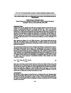
one could lock to the carrier of the satellite signal and obtain much better phase stability but this generally increases receiver complexity and it is the authors’ experience that the C/A code H I T E NOI5E PM - 13 stability is adequate for common-veiw comparisons to under 10 ns. -14 Multipath distortion can be a significant error source and exb” periments have been conducted showing a few nanoseconds 0 deviation from this cause. It is extremely difficult with given 0 Z -15 antenna locations to estimate the size of the multipath effect e A 0 at 1.575 GH;!. This will clearly vary from satellite to satellite and from one antenna location to another. Operationally, if - I 6 -f SV 6 C-V IIERSUREHENT ND15E 0 SV B C-V flERSUREtIEN1 NOI5E the same geometry for viewing the satellite during each sidereal A 5V II C-V tlER5UREHENT N015f A day is used, then whatever multipath distortion is present reBRRUNSCHNEIE-TOKYO PRTH - 17 mains a constant. By keeping the tracking times on a sidereal 4 5 6 7 schedule, which is very convenient for the common-view apLOG T (SECONDS) proach, the multipath instabilities have been found to be of the Fig 1. Fractional frequency stability limitation due to GPS commonview measurement noise for the Braunschweig-Tokyo path. Noise order of 1 ns, so long as the geometrical relationships of refleccomponents are separated for SV 6 , 8, and 11 using the three corner tive surfaces are maintained. The disadvantage, of course, is that hat method. advancing the observation time nominally 4 min each day causes one gradually to move through from nighttime t o daytime ionospheric delays (or vice versa). Fortunately, since these delays typically do not change dramatically, the time error due to such a slow ionospheric walk does not effect frequency comparisons and has only minor effects on time comparisons, unless the baselines are large, i.e., several hour angles.
-
111. ESTIMATEOF COMMON-VIEW MEASUREMENT NOISE Often there are three or more satellites available each day for simultaneous common-view between two sites. Rewriting (3) with the subscripts i, j, or k denoting three different satellites yields three independent measurements (at different times ti, ti, and t k ) of the time difference between clocks at the two sites fAi
-
fBi =
(tL - tb)i + A t D i ,
for i,j, or k.
0
5
-f tlER5UREMENT NOISE
-15
V I R 5V 6
0 IIEASUREMENT NOISE VIR A MERSURMENT NOISE V I R ._
4
4\
SV B 5V 9
BOULDER-TOKYO PRTH 5 6 LOG T (SECONDS)
(5J Fig.
2. Fractional frequency stability due to GPS common-view measurement noise for the Boulder-Tokyo path. Noise components are separated for SV 6 , 8 , and 9 using the three corner hat method.
For the clock sites reported in this paper the time dispersions are only 1-6 ns per day. Also, the satellite passes can usually be time-blocked in a period less than 1 2 h long. Hence, the view paths may then be estimated. Figs. 1-4 are applications dispersion in comparing the difference tAi - tBi with t A . - of this technique. I t for i # j should be less than about 3 ns. One can, therefore, In principle, since the site clocks are also independent, one Bi subtract equations of the form of (5) for i and j from each may subtract the measurement noise variance from the total other, with small error contributions from the site clocks variance for the comparison and thus gain an estimate of the composite variance of the two site clocks. Figs. 5 and 6 illus( t i - t i )1.1.= -At,..‘1 ( 6 ) trate an application of this technique. where the subscript z j denotes the difference taken between the Iv. INTERNATIONAL TIMEAND FREQUENCY two equations (5) for i and j . Equation ( 6 ) also holds for the STANDARDS COMPARISON subscript pairs ik and jk. Taking the variance of ( 6 ) yields A portable clock (PC) has been carried between Washington, for either Q,ik,or jk. a 2 ( t i - th).. SE a$ = a i t o i j , 11 D C and Paris, France to measure the Paris Observatory clock (7) (UTC(0P)) against the U.S. Naval Observatory (USNO) master clock (UTC(USN0-MC)). At 0 8 0 2 UTC September 10, 1983 Since the paths and the satellites are nominally independent, (MJD 45587.3347) is was found that one can solve for individual variances UTC(USN0-MC) - UTC(0P) “51 . l o 1 ps k 0.035 ps ‘ i t D i = 1 / 2 c a % t D1.1. + ‘ a ’ D i k - ‘ADik 2 l (8 1 PC with two other similar expressions with i, j , and k cyclically including relativistic corrections of 23 ns [2]. Concurrent permuted. The measurement noise for each of the common- common-view measurements of GPS satellites were conducted
ALLAN ef al. : INTERNATIONAL TIME AND FREQUENCY COMPARISONS
121
- 12 -
I
2
-13
?
WHITE
L
NUI5E PM
--c
-13
b”
b”-14
0
I
q
0 I
-16
L
0 -14
7
5 6 L O G T (SECONDS)
Fig. 3. Fractional frequency stability of GPS common-view measurements for the Boulder-Paris path via SV #9. Circles indicate composite noise of clocks and the SV #9 common-view link. Pluses are noise of the SV #9 link alone. Slope of white noise PM is shown for reference. -I
WHITE
I
-
I
0
I
NOISE
PM
-1
I
b”
-15
__
5 6 L O G T (SECONDS)
Fig. 6. Fractional frequency stability of GPS common-view measurements for the Boulder-Tokyo path via SV numbers 6,8,and 9. (Common-view link noise removed.)
between NBS Boulder and USNO, and between NBS Boulder and OP, using (electromagnetic) signals from GPS satellites to derive time comparisons. The Sagnac correction from Boulder, CO, to Paris, France, varies from 71 to 1 12 ns and from Boulder to Washington, DC, varies from 11 to 1 3 ns, depending on satellite position. Using the appropriate relativistic corrections for each common-view time difference obtained via GPS NAVSTAR 4 , 5 , and 6 satellites, yields
d
0
UTC(USN0-MC) - UTC(0P)
I 0 0 J
-I