Working Paper No. 02-06-01 Structured Assessment of Risk Systems and Value at Risk (VaR) Joe H. Sullivan Robert Brooks Zachary G. Stoumbos, Ph.D.
I.
Structured Assessment of Risk Systems and Value at Risk (VaR)
Joe H. Sullivan, Ph.D. Mississippi State University
Robert Brooks, Ph.D., CFA The University of Alabama
Zachary G. Stoumbos, Ph.D. Rutgers, The State University of New Jersey
Original date: June 1, 2002 Original Title: Assessing the Accuracy of Value at Risk (VaR) This version: August 30, 2002 Please comment, but do not quote.
CONTACT: Robert Brooks Box 870224 The University of Alabama Tuscaloosa, AL 35487 205.348.8987
[email protected]
Structured Assessment of Risk Systems and Value at Risk (VaR)
An important question for corporate finance officers is whether risk management systems, such as Value at Risk (VaR), currently are producing accurate results. In contrast to previous research on assessing the accuracy of risk systems or VaR, which has focused on backtesting a large sample of historical observations, we provide tools for real-time assessment, using a time window that varies adaptively with the data. The objective is to quickly signal if the estimation process currently is systematically biased, subject to a specified rate of false detections. For example, if the volatility is systematically underestimated by 25% our procedure detects this in an average of 25 observations. Previous techniques have often backtested thousands of observations. We also discuss the trade-off between increasing detection power at the risk of detecting meaningless errors and suggest a parameter to specify the balance desired for a specific application.
Page 1 S t r u c t u r e d As s e s s m e n t o f R i s k S ys t e m s a n d V a l u e a t R i s k ( V a R )
I.
Introduction........................................................................................................................ 2
II.
Assessing the Accuracy of the Estimated VaR .................................................................. 7 A)
Detecting a Single Regime Shift .................................................................................. 14
B)
Detection Power for a Fixed Sample Size with an Uninformative Distribution .............. 17
C)
Detection Power for a Fixed Sample Size with an Informative Distribution .................. 19
III. Example Using Natural Gas Futures Contracts................................................................ 21 A)
Natural Gas Futures Contracts.................................................................................... 21
B)
Alternative Estimates of Volatility................................................................................. 23 i)
Centered and Lagged Moving Averages................................................................... 23
ii)
GARCH(1,2) ............................................................................................................. 24
iii) OLS Regression with Trigonometric Basis Functions................................................ 25 C)
A CUSUM Example ..................................................................................................... 27
D)
An Exponentially Weighted, Moving Average Example ............................................... 30
IV. Conclusion ....................................................................................................................... 32 V.
References ...................................................................................................................... 42
VI. Appendix Alternative Distributions.................................................................................... 34 i)
The 2-Normal Distribution ......................................................................................... 34
ii)
The One-Parameter Beta Distribution....................................................................... 35
iii) The 2-Step Uniform Distribution................................................................................ 36 iv) The Linear-Uniform Distribution ................................................................................ 38 v)
Comparison of the Alternative Distributions .............................................................. 40
Page 2 S t r u c t u r e d As s e s s m e n t o f R i s k S ys t e m s a n d V a l u e a t R i s k ( V a R )
Structured Assessment of Risk Systems and Value at Risk (VaR)
II.
Introduction Bank and corporate finance executives are implementing enterprise risk
management systems to better understand and manage a firm’s risks. Our objective is to provide tools that evaluate in real-time the current accuracy of these systems, in contrast with previous research which has focused on backtesting a large historical sample, often data for several years. We provide tools quickly assess whether there is a systematic bias in the recent past. We are able to detect moderate systematic bias in as few as 25 observations when the portfolio volatility is estimated to be 75% of its true volatility. In contrast, previous methods often envision backtesting a fixed sample size that often runs in the thousands of observations. In many situations waiting to accumulate thousands of daily observations before testing for systematic bias is a very long time to wait. Especially in markets where the risks are large and complex, it is crucial to establish the accuracy of the risk system and verify that there is no systematic bias currently present in the process. Often, firms are so pleased to finally have an enterprise risk management system in place that they forget to address whether the resulting daily risk assessment has any legitimacy. The ability to certify that a system is without significant bias is useful for building confidence in the risk-management decision-making process. Also, there is a direct feedback loop between theoretical market models and valuation models used within these systems and certifying the system. It is possible to identify superior market
Page 3 S t r u c t u r e d As s e s s m e n t o f R i s k S ys t e m s a n d V a l u e a t R i s k ( V a R )
models and superior valuation models through the effort of system certification. Although we focus in this paper on value at risk, the methodologies developed are directly applicable to many other risk measures. Portfolio risk is most comprehensively captured in the distribution for the change in portfolio value over some specified unit of time. VaR is estimated by a single point of that distribution. Thus, the purest assessment of VaR estimation accuracy is whether the observed change has the specified violation probability, conditioned on the recent history. A much more powerful test, which requires fewer observations for the same detection probability, results from using the entire estimated distribution for the change in portfolio value. However, much of the increased power may result from detecting errors in the distribution that are not relevant to the VaR estimation. We suggest a compromise between testing only the relevant point of the distribution and detection power. Value at risk (VaR) is concerned with the risk of loss. The VaR’s focus is on the distribution of possible outcomes. Specifically, VaR measures the maximum loss over a stated time period, under normal market conditions at a pre-specified confidence level. By analogy, VaR is a good measure of storm intensity, but it is not intended to measure damage from hurricanes. That is, VaR measures the damage from moderately rare events (say one out of 20 outcomes), rather than very infrequent events such as 100year floods or powerful hurricanes. For more information on the basics of VaR, see Beckstrom (1995), Beder (1995), Jorion (1997), Dowd (1998), Best (1999), and Hull (2000).
Page 4 S t r u c t u r e d As s e s s m e n t o f R i s k S ys t e m s a n d V a l u e a t R i s k ( V a R )
Typically, VaR is modeled with a probability distribution for the change in portfolio value over a specified time period, such as a day or a week, and is expressed as a statement of the following form: “We are C percent certain that we will not lose more than V dollars in the next N days.” The value at risk is V and depends on the confidence level C and the time period N. The confidence level C may be expressed alternatively as (1 – α) 100%, so that, for example, a confidence level of 95% corresponds to α = 0.05. Basak and Shapiro (2001) give as the standard definition of VaR that value V such that Pr( − X i ,N ≤ V ) = 1 − α , α ∈ [0,1] ,
(1)
where W i is the portfolio value or wealth at time i, X i ,N = Wi − Wi −N is the gain in portfolio value for N periods ending with period i, and − X i ,N is the loss of wealth. The Basak and Shapiro (2001) formulation includes infallible portfolio insurance at some floor value W , meaning that Pr(Wi < W ) = 0 ⇒ Pr(Wi −N − Wi ≤ V = Wi −N − W ) = 1 , so that α = 0 implies that VaR is Wi −N − W . When α = 1 the VaR constraint is never binding. The relationship above is equivalent to (2)
Pr( X i , N < −V ) = α ,
so that –V is the α quantile of the distribution for X i , N . If the distribution of portfolio returns is normal with zero mean and volatility σ iWi −N , and Zα is the α quantile of the standard normal distribution, then the VaR is V = Wi− N σ i Zα . Although a premier virtue of VaR is in its simplification of the complexities of risk management, Basak and Shapiro (2001) argue that the simplification may have been
Page 5 S t r u c t u r e d As s e s s m e n t o f R i s k S ys t e m s a n d V a l u e a t R i s k ( V a R )
carried too far. They construct a model in which agents optimize their own utility subject to a risk constraint specified in terms of VaR. Because the VaR constraint fails to consider the degree of violation, these agents are induced to favor excessive risktaking. In their model, the agents purchase insurance against mild violations of VaR so that the specified violation probability is honored, but the distribution of losses is shifted toward large losses in the event of a violation. Typically, VaR is estimated at the close of every trading day. If the VaRestimation process is accurate, then the probability of loss exceeding the VaR should be α. Christoffersen (1998) develops a method for testing the violation probability, or coverage, in a historical sample, as well as the independence of the violations. He points out that the VaR violations may cluster so that the conditional violation probability may differ from the specified value even if the unconditional coverage is correct. Thus, he tests for accurate conditional coverage, which is composed of independent tests for unconditional coverage and independence. Since VaR is typically estimated as a specified quantile of an estimated density forecast, Diebold, Gunther, and Tay (1998) discuss evaluating the accuracy of the estimated density for the portfolio gain corresponding to the VaR time horizon, testing the sequence of density forecasts for shape and anticipation of volatility clustering in the observations. They illustrate their idea with simulated data and a series of four increasingly accurate forecasting methods that demonstrate all four possibilities of accuracy or inaccuracy in the shape and clustering. Christoffersen and Diebold (2000) contend that the extent of volatility clustering and, by extension, VaR violation clustering depends on the time horizon. They conclude
Page 6 S t r u c t u r e d As s e s s m e n t o f R i s k S ys t e m s a n d V a l u e a t R i s k ( V a R )
that if the time horizon is more than ten to twenty trading days (depending on the asset) there is little difference between the conditional and unconditional volatility forecasts. They use a constant 2-sigma interval about the unconditional mean, using the unconditional standard deviation, defining a “hit sequence” that is 1 if the observation falls within the 2-sigma interval and 0 otherwise. They use a non-parametric runs test for independence in the hit sequence, testing four equity indexes and four foreign exchange rates with 6,350 historical observations from each market. The observed level of significance for the null hypothesis of independence depends on the level of aggregation, always being significant for daily observations. They generally reject independence for aggregation of less than ten trading days and conversely for horizons greater than ten days Berkowitz and O’Brien (2002) apply the testing framework of Christoffersen (1998) to bank data, concluding that the unidentified large banks were generally conservative in their VaR estimation and two of the banks had significant first-order autocorrelation in the VaR violations. Berkowitz (2001) introduces a different model for testing the density forecasts underlying the VaR estimates. Berkowitz (2002) considers a multifactor pricing model for the portfolio valuation and shows how to distinguish between errors in the pricing model and the multivariate density forecast of the pricing factors. Christoffersen (1998), Berkowitz (2001), and Berkowitz and O’Brien (2002) focus on backtesting two aspects of VaR accuracy, the unconditional coverage and correlation. Simply testing whether the overall frequency of VaR violations approximates the specified value requires a very large amount of data, because violations are
Page 7 S t r u c t u r e d As s e s s m e n t o f R i s k S ys t e m s a n d V a l u e a t R i s k ( V a R )
typically specified to be rare. Including the distribution used in the VaR estimation process, or its lower tail, greatly increases the detection power, making feasible the use of smaller sample sizes. The second aspect is clustering of VaR violations. For example, portfolio returns may exhibit volatility clustering, which is not adequately represented in the VaR estimation process, with the result that VaR violations are also clustered, although the violation rate may be correct when averaged over a long period. We consider the related problem of assessing the VaR estimation process in real-time, without waiting for the accumulation of a historical sample. We model a regime shift, in which the VaR estimation process at some point becomes systematically biased, which should be detected promptly. We also note the increase in detection power as more of the density forecast is used. Several additional backtesting procedures are identified and their power compared with a sample size of 125 observations.
III.
Assessing the Accuracy of the Estimated Distribution and VaR Let wi represent the known historical value observed at time i and
X i ,N = Wi − w i −N represent the increase in portfolio value from i - N to i, given Ψi− N , the information-set at time i - N. For one-period changes, we simplify the notation to X i ≡ X i ,1 . Thus, X i ,N = X i + X i −1 + K + X i −N +1 is an MA(N - 1) process. The autocovariance is γ i , j ,N = E (( X i ,N − E ( X i ,N )) * ( X i − j ,N − E ( X i − j ,N ))) = E ( X i ,N X i − j ,N ) if the means are zero. Generally, the process {X i } will not be covariance stationary, which would require γ i , j , N = γ i +t , j +t , N for all values of t. Under the further assumption that one-
Page 8 S t r u c t u r e d As s e s s m e n t o f R i s k S ys t e m s a n d V a l u e a t R i s k ( V a R )
period changes are uncorrelated, γ i , j ,N = σ i2− j + σ i2− j −1 + K + σ i2−N +1 for 0 ≤ j < N , and 0 otherwise. The autocorrelation is ρ i , j ,N = γ i , j ,N / γ i ,0,N , with ρ i , j ,N ≈ Max (N − j , 0) / N for slowly changing variance σ i2 . = E (( X i ,1 ) 2 ) . Let the true cumulative distribution function (cdf) for X i ,N given Ψi −N be a continuous function Gi ,N , meaning that Gi ,N ( x ) = Pr( X i ,N ≤ x | Ψi −N ) , and let the estimate of Gi ,N be Fi ,N , also assumed to be continuous. The notation simplifies for N = 1 to Gi = Gi ,1 and Fi = Fi ,1 . Thus, the “true” VaR for time i, estimated at i - N, is Vi ,N = −Gi−,N1 (α ) , since Pr( X i ,N ≤ −Vi ,N ) = α
⇒ Gi ,N ( −Vi ,N ) = α
⇒ Vi ,N = −Gi−,N1 (α ) . The
“estimate” of VaR is Vˆi ,N = −Fi ,−N1(α ) . The random variable Gi ,N ( X i ,N ) follows a Uniform(0,1) distribution, since the probability that it is less than or equal to some value u is just u, for 0 ≤ u ≤ 1 . To see that this is true, note that Pr (Gi ,N ( X i ,N ) ≤ u ) = Pr ( X i ,N ≤ Gi−,N1 (u )) = Gi ,N (Gi−,N1 (u )) = u , for 0 ≤ u ≤ 1 . This suggests testing the distribution of the random variable Ui ,N = Fi ,N ( X i ,N )
as a way of assessing the accuracy of the estimated distribution, with the null hypothesis H0 that Fi,N = Gi,N, i = 1, …, n. For 1-period forecasts U i = U i ,1 . Under the alternative hypothesis H1, Fi ≠ Gi, i ≥ ν , there is a more general expression for the cdf of Ui. By the definition of the cdf, Gi ( x ) = Pr( X i ≤ x ) , so substituting Fi −1(u ) for x gives Gi (Fi −1(u ) ) = Pr( X i ≤ Fi −1(u ) ) . Applying the function Fi to both sides gives Pr( X i ≤ Fi −1(u ) ) = Pr(Fi ( X i ) ≤ Fi (Fi −1(u )) = u ) . Using the definition of Ui = Fi(Xi) gives Pr(Fi ( X i ) ≤ u ) = Pr(U i ≤ u ) . By the definition of the cdf, if a function Hi is the
Page 9 S t r u c t u r e d As s e s s m e n t o f R i s k S ys t e m s a n d V a l u e a t R i s k ( V a R )
cdf of random variable Ui, then H i (u ) = Pr(U i ≤ u ) . Thus, we recognize that the cdf function H i (u ) = Gi (Fi −1(u ) ) . This simplifies to the uniform cdf, Pr(U i ≤ u ) = u, 0 ≤ u ≤ 1, when Gi is the same as Fi. The probability density function (pdf), the derivative of the cdf, is hi (u ) =
g i (u ) =
d d d g (F −1(u ) ) H i (u ) = Gi (Fi −1(u ) ) = g i (Fi −1(u ) ) Fi −1(u ) = i i−1 , where du du du fi (Fi (u ) )
d −1 d −1 Gi (u ) and fi (u ) = Fi (u ) . du du
A practical complication is that U i ,N and U j ,N are correlated unless i − j ≥ N . It is conceptually straightforward to use the conditional distribution of X i ,N | Ψi −1 = X i , which is the same as the N = 1 case. Berkowitz and O’Brien (2002) point out that the Basle Accord permits the use of VaR estimates for setting bank capital requirements, using the N = 1 case and α = 0.01. Other applications of VaR use a longer time interval than one day. For example, Hull (2000) refers to a 10-day VaR in setting bank capital requirements. Nevertheless, even for a multiple period VaR, most of the effort in estimating VaR lies in estimating the function Gi ,N . Once the function is estimated, it should be simple to adjust Gi ,N . slightly to get Gi = Gi ,1 , the distribution for the portfolio gain for the first day of the period. Thus, we will simplify the notation to N = 1. Several authors have noted the lack of power in direct testing of VaR violations. For example, a series of daily 99% VaR estimates would be expected to have about 2.5 violations in the 250 or so trading days in a calendar year. It would require a sample of several years to have adequate power in detecting a conservative bias. On the other hand, using the probability integral transformation applied to the observed portfolio gain
Page 10 S t r u c t u r e d As s e s s m e n t o f R i s k S ys t e m s a n d V a l u e a t R i s k ( V a R )
increases the detection power but at the cost of detecting errors in parts of the density that are not relevant to risk assessment. We point out an intermediate method that uses a specified part of the forecast distribution. Since the VaR is the α quantile of the estimated distribution, define a neighborhood δ ≥ 0 such that the estimated distribution is used if the transformed variable Ui is within the δ-neighborhood of α and 0 or 1 otherwise. Specifically, define a modified transformation
u i ,α ,δ
x i < Fi −1(α − δ ) 0, = u i = Fi −1( x i ), Fi −1(α − δ ) ≤ x i ≤ Fi −1(α + δ ) 1, otherwise.
This has the density function (pdf)
hi ,α ,δ (u ) =
d P(U i ,α ,δ du
≤ u) =
0, H i (α − δ ) /(α − δ ),
u≤0 0 < u ≤α −δ
hi (u ),
α −δ < u ≤α +δ α +δ < u ≤1 1< u
(1 − H i (α + δ )) /(1 − α − δ ), 0,
for the case 0 < α − δ < α + δ < 1. The specifications for α < δ and 1 < α + δ are straightforward but omitted for brevity. Under this model, the degree of loss is considered in the likelihood only for losses in a neighborhood of VaR. This transformation corresponds to the Christoffersen (1998), Christoffersen and Diebold (2000) and Berkowitz and O’Brien (2002) hit sequence when δ = 0, and the uniform transformation of Diebold, Gunther and Tay (1998), Berkowitz (2001), and Berkowitz (2002) when δ = 1. This allows for an explicit compromise between using only the single
Page 11 S t r u c t u r e d As s e s s m e n t o f R i s k S ys t e m s a n d V a l u e a t R i s k ( V a R )
point of the density that specifies VaR (high relevance but low power) and using the entire estimated density (low relevance but higher power). In many VaR applications, handling volatility clustering is a major challenge in achieving accurate VaR calculation. As Christoffersen and Diebold (2000) point out, volatility clustering is “an inherently symmetric phenomenon,” and they include the upper tail of the distribution. Our transformation can use both tails of the estimated distribution with this definition
u i ,α ,δ ,2
=
0,
x i < Fi −1(α − δ )
ui ,
Fi −1(α − δ ) ≤ x i ≤ Fi −1(α + δ )
.5,
Fi −1(α + δ ) ≤ x i ≤ Fi −1(1 − α − δ )
ui ,
Fi −1(1 − α − δ ) ≤ x i ≤ Fi −1(1 − α + δ )
1,
otherwise.
This has the density function (pdf) hi ,α ,δ ,2 (u ) =
0, H i (α − δ ) /(α − δ ),
u≤0 0 < u ≤α −δ
hi (u ),
(1 − H i (1 − α + δ )) /(α − δ ),
α −δ < u ≤ α +δ α + δ < u ≤ 1− α − δ 1− α − δ < u ≤ 1− α + δ 1− α + δ < u ≤ 1
0,
1< u
(H i (1 − α − δ ) − H i (α + δ )) /(1 − 2α − 2δ ), hi (u ),
for the case 0 < α − δ < α + δ < 1 − α − δ < 1 − α + δ < 1 . The specification for other cases is straightforward and omitted for brevity. An example two-tailed distribution where the true variance exceeds the estimated variance is given in Figure 1, using the values 0.25 and 0.10, respectively, for α and δ.
Page 12 S t r u c t u r e d As s e s s m e n t o f R i s k S ys t e m s a n d V a l u e a t R i s k ( V a R )
Figure 1 Example of a two-tailed, high-variance distribution for Ui, α = 0.1, δ = 0.05. 2 1.8 1.6 1.4 hi (u )
1.2 1
0.8 0.6 0.4 0.2 0 0
0.2
0.4
0.6
0.8
u
1
The infinitely many ways that the null hypothesis can be violated can be classified broadly into systematic biases for which the distribution for Ui has increased probability near the mean so that the variance of Ui is less than the that of the uniform distribution and those with decreased probability near the mean (and having a higher variance). This classification is illustrated by the three example distributions shown in Figure 2. One specific alternative distribution, adjusted for α and the specified neighborhood δ, will be used in a likelihood test. We consider several specific functions to capture systematic bias. First, we note the possibility of semantic confusing between the variance of Ui and the variance of the portfolio return. If the true portfolio variance
Page 13 S t r u c t u r e d As s e s s m e n t o f R i s k S ys t e m s a n d V a l u e a t R i s k ( V a R ) ∞
(the variance of Gi,
∫ (x − µ
G
)dGi ) is larger than the estimated variance (the variance of
−∞ ∞
Fi,
∫ (x − µ
F
)dFi ), then Ui will have greater variance than the uniform (0,1) distribution.
−∞
Figure 2 Three alternative distributions for Ui 0.25
Pr@Ui ≤ uD
0.2
higher variance
0.15
uniform
0.1
0.05
lower variance
0 0
0.05
0.1 u
0.15
0.2
The best testing scheme for detecting violations of the null hypothesis depends on the specific alternative distribution. Thus, it is important to characterize the distribution that may hold for Ui, when the value at risk distribution is not accurately estimated. We consider four families of distributions for Ui. The first family, which we call the "2-Normal" distribution, is obtained when Gi and Fi are normal with mean zero, so the only inaccuracy is in estimating the volatility. The single parameter for this distribution is η 2N ,i = σˆ i / σ i , the ratio of estimated to true volatility. This distribution is similar in shape to the beta distribution with the shape and scale parameters constrained to take the same value, η β . Using the entire distribution corresponds to δ =
Page 14 S t r u c t u r e d As s e s s m e n t o f R i s k S ys t e m s a n d V a l u e a t R i s k ( V a R )
1. We also considered an uninformative distribution that is uniform at one of two values, called the "2-step uniform" distribution, which corresponds to α = 0.20 and δ = 0. The incremental probability is constant over the interval (0, 0.2) and constant at a different value over the interval (0.2, 1). The single parameter is η2U = Pr(Ui ≤ 0.2) . We also have a family where only observations in the lower-tail are informative, the "linearuniform" distribution, which corresponds to α = δ = 0.10. This distribution also has a single parameter ηLU = Pr(Ui ≤ 0.2) . The incremental probability varies linearly over (0, 0.2) and is constant over (0.2, 1). These distributions are described in detail in the Appendix.
A. Detecting a Single Regime Shift Several different settings are possible for assessing VaR accuracy. The two most common perspectives are testing a historical sample of fixed size (backtesting) and sequential testing with a decision after each new observation. We will first consider the sequential testing setting, with the further simplification that there is a single regime shift to the alternative hypothesis (H1) distribution at some unknown location ν, which may be infinite. Thus, a shift to H1 is persistent and is to be detected as quickly as possible, subject to some specification of false detection probability. The simplest alternative distribution is one that is fully specified, so that there are only two possibilities the null hypothesis (H0) of accurate estimation for which Hi is the uniform distribution or the alternative hypothesis (H1) that Hi remains fixed at some specific other distribution that is known. It turns out that a test that works well in
Page 15 S t r u c t u r e d As s e s s m e n t o f R i s k S ys t e m s a n d V a l u e a t R i s k ( V a R )
detecting a specific alternative distribution also works well for a family of similar distributions. It is simpler, however, to focus on a single specific distribution. Page (1954) proposed a powerful class of sequential tests based on the score statistic Ci = ln(hi ,1 (U i ) / hi , 0 (U i )) , which is the logarithm of the likelihood ratio statistic for observation Ui. The functions hi,0 and hi,1 are the probability density functions hi for Ui under the null (H0) and alternative (H1) distributions, respectively. Lai (1995) summarized the CUSUM and its properties, noting that the test signals a regime shift at m observation M = inf m : max ∑ Ci ≥ cγ . Observation k is an estimate for the location 1≤ k ≤ n i = k of the first shifted observation, although not the likelihood maximizing estimate. Page referred to this as a cumulative sum (CUSUM) test since the score statistics are summed. The critical value cγ can be specified indirectly by requiring that the expected value of M, which is called the average run length or ARL, be γ when the shift location is infinite (no shift). The CUSUM test is optimal in the sense of having the smallest expected number of shifted observations to signal. Moustakides (1986) and Ritov (1990) demonstrated this optimality. Let ℑγ be the class of all tests with ARL ≥ γ when all observations are from the null distribution. When there is a regime shift beginning with observation ν < ∞, we want to consider the expected detection delay = E(T – (ν – 1) for a test T ∈ ℑγ, but considering only positive values and conditioning on the shift location and the observations before the shift. Thus, we want to minimize the conditional expected detection delay Tν , X = E ((T − ν + 1)+ | X1,K, Xν −1) for a test T ∈ ℑγ. The CUSUM minimizes the worst-case conditional expected detection delay,
Page 16 S t r u c t u r e d As s e s s m e n t o f R i s k S ys t e m s a n d V a l u e a t R i s k ( V a R )
E1(T ) = sup ess sup(Tν , X ) . Stoumbos et al. (2000) also discuss the CUSUM, as well as 1≤ ν
Bayesian procedures that could be used if there is prior knowledge about the shift location. The optimality of the CUSUM applies only to one specific distribution, but it is effective in detecting shifts to similar distributions. So, for example, a CUSUM test that was optimized for a Beta(1.5, 1.5) alternative distribution hi,1 would be effective in detecting any one-parameter beta distribution with a parameter value greater than 1.5. The effectiveness would diminish as the parameter approached 1, and the test would be ineffective with parameter values below 1. This is referred to as a “one-sided” CUSUM test because it is effective in detecting only one side of the interval of possible parameter values. For a practical application, both increased- and decreased-variance alternative distributions need to be detected. One approach is to combine two CUSUM tests. One is designed to be sensitive in detecting the family of increased-variance distributions. The other is designed for detecting the family of decreased-variance distributions. If either test signals, that is a signal for the overall test, which is sensitive to a shift to either family of distributions. The performance is measured by the worst-case conditional expected delay, which is estimated from simulation. To illustrate the performance, two one-sided CUSUM tests were constructed for the 2-normal alternative distribution with parameter values of 1.3 and 1/1.3. Simulation was used to estimate a critical value of 2.6 used in each one-sided CUSUM, which gave an overall Average Run Length (ARL) of approximately 125 with observations from the null distribution.
Page 17 S t r u c t u r e d As s e s s m e n t o f R i s k S ys t e m s a n d V a l u e a t R i s k ( V a R )
Figure 3 shows the ARL when the VaR distribution is inaccurate, with the inaccuracy parameterized by the ratio of estimated to actual volatility. The ARL values were estimated from simulation with 1000 repetitions. Figure 3
ARL
Average run length of two one-sided CUSUM tests
120 100 80 60 40 20 0 0.7
0.8
0.9 1 1.1 1.2 Estimated : Actual Volatility
1.3
1.4
B. Detection Power for a Fixed Sample Size with an Uninformative Distribution Backtesting a fixed sample of n observations is a different setting. With sequential testing, where a decision is rendered after each new observation, the CUSUM is optimal and should be used instead of applying a fixed-sample test to a moving window of recent observations. The detection power, the probability of rejecting H0: Ui ~ Uniform(0,1), i = 1, …, n, with n = 125 observations from the 2-step uniform distribution, is shown for different parameter values in Figure 4. With an uninformative
Page 18 S t r u c t u r e d As s e s s m e n t o f R i s k S ys t e m s a n d V a l u e a t R i s k ( V a R )
alternative distribution, the simple proportion test, labeled "proportion”, should, and does, do well. This test statistic is the number of observations less than or equal to 0.2. The critical values are the 0.0243 and 0.980 quantiles of the binomial(n, 0.2) distribution, 16 and 34. This test has the greatest power among those shown. A modified version of the Kolmogorov-Smirnoff test, labeled “KS”, was evaluated. The test statistic was the maximum deviation of the sample cdf from the uniform distribution, but only taking the maximum over the lower 20% of the cdf. The critical value was estimated as 0.0799 using simulation. This test is effective for η2U < 0.2 and has intermediate power for η2U > 0.2. The test labeled “betaMLE” uses the test statistic Abs( ηˆβ -1), where ηˆβ is the maximum likelihood estimate (MLE) for the Beta(ηβ, ηβ ) distribution. The critical value for this test statistic was 0.2163, estimated from simulation as the 0.95 quantile of the null test statistic distribution. This test is slightly biased, with a minimum signal probability of approximately 0.03 for η2U = 0.225, and it is the least powerful test among those shown when the observations are from the uninformative distribution. The last test shown is based on the lower 20% of the observed distribution. The smallest 0.2 n = 25 observations are selected and then multiplied by 5 (but limited to a maximum value of 0.99). Then, the resulting values were converted to quantiles of the standard normal distribution. The absolute value of the usual t-test statistic, 5 * mean / (standard deviation), was the test statistic. The critical value was estimated from simulation as 0.001138. The adjusted t-test does well but is not quite as powerful as the proportion test.
Page 19 S t r u c t u r e d As s e s s m e n t o f R i s k S ys t e m s a n d V a l u e a t R i s k ( V a R )
A fixed sample size test is useful for testing historical VaR observations, and can be adapted to test current observations by taking a moving window of the n most recent observations for the test. For best results, though, the fixed sample size tests should be adapted for the possibility of a regime shift. Figure 4 Fixed sample size detection power with 125 observations from the 2-step uniform distribution 1
Detection Probability
0.8
0.6
0.4
0.2
0 0
0.05
0.1
0.15
0.2
0.25
0.3
0.35
0.4
η = Pr[U i ≤ 0.2]
proportion
KS
betaMLE
t_adj
C. Detection Power for a Fixed Sample Size with an Informative Distribution The detection power is strongly influenced by the distribution of the observations. With the 2-step uniform distribution, the only information is whether an observation Ui is above or below 0.2. In practice, it is often reasonable to assume that Gi is normal and
Page 20 S t r u c t u r e d As s e s s m e n t o f R i s k S ys t e m s a n d V a l u e a t R i s k ( V a R )
choose a normal distribution for Fi. Under this scenario, the observations Ui would follow the 2-normal distribution. Observations from this distribution give the power curves shown in Figure 5. The horizontal axis is the parameter of the 2-normal distribution η 2N = (estimated volatility) / (actual volatility). In addition to the four tests described above, this figure shows the power for a likelihood ratio test based on the 2normal distribution, labeled “2-Normal”. The 2-Normal test power is similar to that of the betaMLE test. The betaMLE test is slightly asymmetrical, having slightly greater power for 1 < η2N. Figure 5 Fixed sample size detection power with 125 observations from the 2-normal distribution 1
Detection Probability
0.8 0.6 0.4 0.2 Estimated / Actual Volatility
0 0.7
0.8 2Normal
0.9
1 betaMLE
1.1 t_adj
1.2
1.3
proportion
1.4 KS
Page 21 S t r u c t u r e d As s e s s m e n t o f R i s k S ys t e m s a n d V a l u e a t R i s k ( V a R )
IV.
Example Using Natural Gas Futures Contracts
A. Natural Gas Futures Contracts Natural gas is a primary energy source that is gaining in popularity for more than just winter heating. The use of natural gas goes back at least 2,000 years, when the Chinese piped natural gas with bamboo poles from shallow wells to generate heat to separate salt from salt water. By 1996, world natural gas consumption had reached 82 trillion cubic feet, and it is expected to be the fastest growing primary energy source over the next 20 years. U. S. natural gas consumption in 1996 was over 22 trillion cubic feet or approximately 25 percent of total gas consumption. Within the U. S., consumption of natural gas is broken down into the following sectors: 41 percent industrial, 24 percent residential, 14 percent commercial, 12 percent electric utilities, and other sectors consume 9 percent. According to the Oil & Gas Journal, proven world natural gas reserves as of January 1, 2000 are approximately 5,146 trillion cubic feet or a 62-year supply at current consumption levels. Proven reserves have more than doubled over the past 20 years. (See Energy Information Administration 1998 and 2000.) Natural gas is measured in cubic feet (cf) or in British thermal units (Btu). One cubic foot of natural gas is approximately equivalent to 1,000 Btu. Prices are quoted in dollars per million Btu (MMBtu). Henry hub natural gas futures contracts traded on the New York Mercantile Exchange are for 10,000 million Btu (10,000 MMBtu) delivered at Sabine Pipe Line Company’s Henry Hub in Louisiana. Physical delivery takes place over an entire month and the last trading day is three business days before the first
Page 22 S t r u c t u r e d As s e s s m e n t o f R i s k S ys t e m s a n d V a l u e a t R i s k ( V a R )
calendar day of the contract month.1 The natural gas futures price depends on the delivery location. Our data set is based on delivery at the Henry hub. Natural gas futures prices were obtained from Bloomberg from April 3, 1990 through July 30, 2001. Figure 6 illustrates the behavior of the monthly nearby futures market. The quoted futures price is based on daily prices for the next month. Hence there is generally slightly less volatility in the futures prices than in spot prices. From this history, we see evidence of seasonality in prices with the winter season, when consumption of natural gas is high, marked by high prices and high price volatility. In recent years, the summer season has also experienced a milder peak in prices and volatility. Figure 6 Nearby futures prices April 3, 2000 through July 30, 2001 $12
NG Nearby Futures Price
Price per MMBtu
$10 $8 $6 $4 $2 $0 4/1/2000
1
7/1/2000
9/30/2000
12/30/2000
4/1/2001
For more information on natural gas futures contracts, see www.nymex.com.
7/1/2001
Date
Page 23 S t r u c t u r e d As s e s s m e n t o f R i s k S ys t e m s a n d V a l u e a t R i s k ( V a R )
B. Alternative Estimates of Volatility In estimating the distribution of changes in natural gas future prices, estimating the volatility is the most important task. We will consider several alternative ways of estimating the current volatility from the recent history, as a way of generating the distribution used to calculate the VaR. Then, we will demonstrate the VaR assessment tools presented here by applying them to the example VaR estimation processes. i.
Centered and Lagged Moving Averages The expected value of the absolute value of the portfolio gain, | X i |, is σ i 2 , π
provided the gain is normally distributed with mean zero. The moving average of (2T + 1) absolute gains centered about observation i, Ci ,T =
i +T 1 π ∑ abs ( X ) , i 2 j =i −T 1 + 2T
gives an estimate of a time-varying volatility, which is shown in Figure 7. The centered moving average has the disadvantage that it cannot be calculated until T periods after than the current observation. The moving average of (2T + 1) lagged absolute gains, Li ,T =
1 1 + 2T
π i −1 ∑ abs ( X i ) , is available for real-time estimation of the volatility of the 2 j =i −2T −1
next observation. The disadvantage is that if the volatility changes significantly, then this moving average will lag behind the current volatility.
Page 24 S t r u c t u r e d As s e s s m e n t o f R i s k S ys t e m s a n d V a l u e a t R i s k ( V a R )
Figure 7 Volatility estimated from a 25-observation centered moving average NG Volatility Estimates
0.12 0.10 0.08
Abs[gain] 0.06 0.04 C_ma 0.02 0.00 4/1/2000
7/1/2000
9/30/2000 12/30/2000 4/1/2001
7/1/2001
Date
ii. GARCH(1,2) A GARCH(1,2) model was fit to the data according to the model (3)
xi = vi hi
(4)
hi = α 0 + ∑ δ j hi − j + ∑ α j xi2− j
r =1
m=2
j =1
j =1
The error terms vi are independent and identically normally distributed with zero mean and unit variance. The coefficients were estimated by conditional maximum likelihood as α0 = 0.0000735, α1 = -0.0629, α2 = 0.173, δ1 = 0.847, with standard errors, respectively, 0.0000331, 0.0371, 0.0483, and 0.0373. Since the t-statistic for α1 was 1.70, the data do not show that α1 is significantly different from zero. A value of zero was used for α1 in calculating volatility estimates. Figure 8 shows the volatility estimates
Page 25 S t r u c t u r e d As s e s s m e n t o f R i s k S ys t e m s a n d V a l u e a t R i s k ( V a R )
derived from this model, along with the 25-observation lagged moving average of absolute gain. The GARCH model has less delay in responding to changes in volatility and is shown by the line with the sharper peaks. Figure 8 Volatility estimated by a GARCH (1,2) model NG Volatility Estimates
0.12 0.10
Volatility
0.08
Abs[gain]
0.06 garch 0.04 L_ma
0.02 0.00 4/1/2000
7/1/2000
9/30/2000 12/30/2000 4/1/2001
7/1/2001
Date
iii. OLS Regression with Trigonometric Basis Functions Since the variation in volatility is periodic, with the principal peak in the winter and a milder peak in the summer, an alternative fit is provided by the first few terms of a Fourier series. The OLS model (5) abs( xi )
12 12 π = α 0 + ∑ α j Sin(2 π j i / 365.25) + ∑ β jCos(2 π j i / 365.25) + ε i = hˆi + ε i 2 j =1 j =1
was used to estimate the volatility. Since the data are roughly centered on a winter peak, the volatility is approximately an even function and the sine terms are all zero. Only terms with periods of 1, 1/2, 1/6 and 1/7 year were significant, with the resulting
Page 26 S t r u c t u r e d As s e s s m e n t o f R i s k S ys t e m s a n d V a l u e a t R i s k ( V a R )
volatility estimate of
hˆi = 0.0392 + 0.0139 Cos(0.0172 i) + 0.0157 Cos(0.0344 i)
- 0.00581 Cos(0.103 i) - 0.00525 Cos(0.120 i). The OLS trigonometric estimate matches the centered moving average very well, as shown in Figure 9. The trigonometric estimate does not suffer from the lag, but it is not available for real-time estimation, because it is estimated from the entire data set. Of course, one could fit a trigonometric series to recent observations and obtain a useful predictor for the next day's volatility. However, this does not give accurate volatility estimates because the location and magnitude of the peak vary from year to year, and are not easy to predict from recent history. Figure 9 Volatility estimated by trigonometric series 0.12
NG Volatility Estimates
GARCH
0.10
C ma
Volatility
0.08 0.06
Trig
0.04 0.02 0.00 4/1/2000
7/1/2000
9/30/2000
12/30/2000
4/1/2001 Date 7/1/2001
Page 27 S t r u c t u r e d As s e s s m e n t o f R i s k S ys t e m s a n d V a l u e a t R i s k ( V a R )
C. A CUSUM Example We will demonstrate the use of two one-sided CUSUM detection tests by starting with a VaR estimation process that is not very accurate. We will use the 25-day lagged moving average to estimate the volatility, and hence the VaR, for the next natural gas futures price. The estimated volatility specifies the mean-zero, normal distribution Fi and the transformed observation ui = Fi ( xi ) , where xi is the observed price change. The one-sided CUSUM detecting a high volatility estimate for xi, (corresponding to a low variance in ui) uses the score statistic Ch,i = ln(fh (ui ) / f0 (ui )) = ln(fh (ui )) = ln(r ) − 0.5( −1 + r 2 )zu2i , where zui = Φ −1(ui ) is the standard normal value for ui . The choice of r, the volatility ratio under the alternative hypothesis specifies the error for which the detection performance is optimized. For this example a value of r = 1.3 was chosen. The score statistic for detecting a low volatility estimate is the same except for the choice of r = 1/1.3. The cumulative sums of the score statistics are shown in Figure 10. The critical value for each CUSUM is 2.6, estimated from simulation to give an ARL of 250 for the combined CUSUM, when the volatility is estimated accurately. The one-sided CUSUM for low volatility is plotted in the negative direction. The first observation for which 25-lagged observations are available to estimate the volatility is 5/9/2000. Eleven observations thereafter, on 5/24/2000, the low-volatility CUSUM reaches a value of -2.83, exceeding the critical value and signaling a recent history of underestimating the volatility used to estimate VaR. The realized volatility for these 12 days was 0.0262, while the 25-observation lagged estimates had a mean of 0.0218, for a ratio of estimated/actual of 0.83. The lowvolatility CUSUM indicates a continued underestimation of the volatility until the local
Page 28 S t r u c t u r e d As s e s s m e n t o f R i s k S ys t e m s a n d V a l u e a t R i s k ( V a R )
minimum of -5.58 on 6/8/2000. The realized volatility for the 22 observations 5/9/2000 through 6/8/2000 was 0.0406, while the average of the estimated volatilities was 0.0258, for a ratio of 0.64. Another low-volatility episode is indicated beginning about 9/28/2000, signaled after 12 observations on 10/13/2000, and continuing to a local minimum of –3.35 on 10/25. The low-CUSUM begins another sharp decline about 12/1 which persists until about 12/15 at a local minimum of -7.130. The high-volatility CUSUM signals on 3/2/2001 with a value of 2.70, reaching a peak of 4.57 on 3/19/2001. This positive excursion began on 2/6/2001, for a total of 29 observations. The realized standard deviation was 0.0321, and the average of the lagged estimates was 0.0545, for a volatility ratio of 1.70. The signal was given after 18 observations. Figure 10 Two one-sided CUSUMs, with 25-observation and lagged volatility estimates 6
CUSUM statistic
4 2 0 -2 -4 -6 -8 5/1/00
7/31/00
10/30/00
1/29/01
5/1/01
Date
A simple lagged estimator will systematically underestimate when volatility is increasing and overestimate when it is decreasing. The GARCH and trigonometric
Page 29 S t r u c t u r e d As s e s s m e n t o f R i s k S ys t e m s a n d V a l u e a t R i s k ( V a R )
models of volatility are more accurate, and we also demonstrate the CUSUM technique with these better estimates, which are combined in Figure 11. The thin line shows the GARCH plots, while the thicker line corresponds to the trigonometric model. The highvolatility CUSUM is plotted in the positive direction, while the low-volatility CUSUM is plotted in the negative direction. The trigonometric estimates are sufficiently accurate that the associated one-sided CUSUMs remain within the critical values except for one point. The high-volatility CUSUM exceeds the critical value on 8/18/2000 with a value of -2.64 and nearly reaches the critical value on 3/19/2001 with a value of 2.56. We can recognize that the period from 7/6/2000 through 8/18/2000, with 32 observations, was a period in which the volatility was somewhat overestimated. The standard deviation for these 32 observations was 0.0268, while the average of the corresponding volatility estimates from the trigonometric model was 0.0364, for a ratio of 1.359. For the period 2/21/2001 through 3/19/2001, the standard deviation of the 19 observations was 0.0196, while the average of the volatility estimates was 0.0320, for a ratio of 1.634. The GARCH model is not sufficiently accurate to keep the corresponding CUSUM statistics within the critical values. The high-volatility CUSUM signals on 7/21/2000 and does not begin a persistent decline until about 11/13/2000. Another high volatility signal is given on about 2/28/2001, with the CUSUM statistic continuing to increase until about 5/4/2001.
Page 30 S t r u c t u r e d As s e s s m e n t o f R i s k S ys t e m s a n d V a l u e a t R i s k ( V a R )
Figure 11 CUSUMs for the GARCH and trigonometric models 7
GARCH
6 5
CUSUM statistic
4 3 2 1
Trig
0 -1 -2 -3 -4 5/1/00
7/31/00
10/30/00
1/29/01
5/1/01
Date
D. An Exponentially Weighted, Moving Average Example One simple approach is to test whether the volatility estimate itself is accurate, by comparing it with the absolute value of the gain. If the volatility estimates are accurate, the standardized absolute gain, the absolute value of the gain divided by the estimated volatility, has an expected value of
2 / π . A straightforward way to detect
deviations is to test the exponentially weighted, moving average (EWMA) of the standardized absolute gains. The general form for a series of observations {Yt }t =1 is T
given by Harvey (1989, p. 25) as (6)
mt = (1 − λ )mt −1 + λyt , t = 1, LT ,
Page 31 S t r u c t u r e d As s e s s m e n t o f R i s k S ys t e m s a n d V a l u e a t R i s k ( V a R )
with parameter λ ∈ [0,1]. This recursive relationship can be converted into the explicit sum of past observations t −1
mt = λ ∑ (1 − λ ) j yt − j . j =0
If the observations are independent and have common variance σ Y2 , then the variance of mt is Var (mt ) = λ σ 2
2 Y
t −1
∑ (1 − λ )
2j
j =0
1 − (1 − λ ) 2t λ =λσ = σ Y2σ Y2 (1 − (1 − λ ) 2t ) . 2 1 − (1 − λ ) 2−λ 2
Assuming E(Xi) = 0 E ( | X i | ) = σ X 2
π
2 Y
2
and E ( | X i |2 ) = E ( X i ) = σ X2 . Thus, the
variance of |Xi| is V ( | X i | ) = E ( | X i | 2 ) − ( E ( | X i | )) 2 = σ X2 (1 − 2 ) . If the volatility is π estimated accurately the absolute value of the standardized observed portfolio gain, xi , will have a mean of σˆ i
2
2 π and a variance of (1 − π ) . Using these standardized
values in an EWMA gives (7)
mi = λ
xi 2 + (1 − λ )mi ; m0 = , σˆ i π
. The standard deviation mi is (8)
λ 2i σ mi = 1 − 2 π (1 − (1 − λ ) ) 2−λ
and the expected value is µ m =
2 . Thus, the 3-sigma critical values are µ m ± 3 σ mi . π
The EWMA statistics are plotted with two volatility estimates, one from the GARCH model and the other from the trigonometric OLS model. A smoothing parameter value
Page 32 S t r u c t u r e d As s e s s m e n t o f R i s k S ys t e m s a n d V a l u e a t R i s k ( V a R )
λ = 0.05 is used for this and all other EWMA examples. The plot is shown in Figure 12. Both models estimate the volatility with sufficient accuracy to keep the EWMA statistic within the critical values over the range of observations. Figure 12 EWMA chart with GARCH and trigonometric estimates of volatility 1.2 1.1
Trig
EWMA statistic
1 0.9 0.8 0.7 0.6
GARCH
0.5 0.4 5/1/00
V.
8/1/00
11/1/00
2/1/01
5/4/01
Date
Conclusion The value at risk is defined by the lower limit of a one-sided prediction interval,
with the specified confidence level, such as 95%, being the probability that the observed change in portfolio value falls within the prediction interval. Thus, a simple and direct way of assessing the VaR estimation process is to observe the proportion of changes in value that violate the estimated VaR. Thus, if the VaR process were operating at the 95% confidence level, say, then the test would be how close the proportion of violations was to 5%. We tested several assessment procedures for a specific confidence level of 80% and found their effectiveness was less than that of
Page 33 S t r u c t u r e d As s e s s m e n t o f R i s k S ys t e m s a n d V a l u e a t R i s k ( V a R )
alternative procedures. These more effective alternative procedures are based on a transformation of the observed change in portfolio value, namely the observed value converted into the probability of a value less than what was observed. These probabilities have a Uniform (0, 1) distribution when the VaR process is accurate. We classified the inaccuracies into two categories, those for which the probabilities cluster too near the mean (low variance) and those with high variance. With this classification, we constructed a one-sided test for each category, in the sense that the one-sided test for low variance was effective in detecting only inaccuracies leading to a low variance, and similarly for the high-variance one-sided test. Combining the two one-sided tests gave a test effective in detecting problems leading to either low or high variance. We propose using the log of the likelihood ratio of the observed quantiles as the score statistic for the one-sided test. The expected number of observations required to detect a flawed process depends on the severity of the flaw. If both the true and estimated distributions are normal with mean zero, then one measure of inaccuracy is the ratio of estimated to actual volatility. A ratio of unity represents an accurate VaR process, and deviations from unity are to be detected quickly. We found that, with an average run of 125 observations between false detections, if the estimated volatility was 30% or more too great then the problem was detected in an average of 36 observations. With a volatility ratio of 77% or less, the detection required an average of 27.6 observations. Sometimes it is useful to assess the accuracy of a historical sample. We found that the best procedures, which were based on the likelihood ratio, had a detection probability of approximately 97.7% for a fixed sample size of 125 observations when the
Page 34 S t r u c t u r e d As s e s s m e n t o f R i s k S ys t e m s a n d V a l u e a t R i s k ( V a R )
variance ratio was either 1.3 or 1/1.3 = 0.77, with a specified false detection probability of 5%.
Appendix
Alternative Distributions There are several families of distributions that logically could be considered for modeling the alternative distribution, which we will describe in turn. i.
The 2-Normal Distribution Often it is assumed that the distribution Gi is normal, and it is assumed to have a
zero or negligible mean, due to the small time increment, hedging, or both. Thus, the estimation error is largely due to mis-estimating the volatility. If both Gi and Fi are normal with mean zero, then the distribution Gi o Fi −1 is defined by a single parameter,
η2 N = η2 N ,i = σˆ i / σ i , where σ i is the volatility of the true distribution Gi and σˆ i is the volatility of the estimated distribution Fi. We refer to this distribution as the “2-normal” distribution. For this distribution, the variance of Ui is inversely related to η 2N, with 0 < η 2N < 1 corresponding to a variance higher than that of the uniform distribution, while 1 < η 2N corresponds to a lower variance. The distribution reduces to the Uniform (0,1) when η 2N = 1. Using Φ( z ) =
1 2π
z
∫e
− 0.5 t 2
dt , which is the cdf for the
−∞
standard normal distribution, we can express Gi and Fi as Gi (g ) = Pr(G ≤ g ) = Φ(g / σ i )
Page 35 S t r u c t u r e d As s e s s m e n t o f R i s k S ys t e m s a n d V a l u e a t R i s k ( V a R )
and Fi −1( p ) = σˆ i Φ −1( p ) . Thus, the 2-normal cdf is Pr(U ≤ u ) = Gi (Fi −1(u )) = Φ(Φ −1(u )σˆ i / σ i ) = Φ(η2N ,i Φ −1(u )) . The pdf is 2 φ (η2N ,i zu ) ∂ −0.5 z 2 (η −1) = η2N ,i e u 2N ,i , where zu = Φ −1(u ) is the standard Pr(U ≤ u ) = η2N ,i ∂u φ ( zu )
normal value corresponding to u. The 2-normal pdf is illustrated in Figure 13 with two alternative values for the parameter, η 2N = 1.3 and 1/1.3. The “2Normal” test statistic is the larger of the mean scores, using the 2-normal distribution with parameter values 1.3 and 1/1.3 for f1. The critical value of -0.00354 was estimated from simulation. Figure 13 The 2-normal pdf 2 1.75
η 2N = 1/1.3
1.5
F@uD
1.25 1
η 2N = 1.3
0.75 0.5 0.25 0
0.2
0.4
0.6
0.8
1
u
ii. The One-Parameter Beta Distribution Another single parameter distribution with shape similar to the 2-normal distribution is the beta distribution with both parameters constrained to be the same, the
Page 36 S t r u c t u r e d As s e s s m e n t o f R i s k S ys t e m s a n d V a l u e a t R i s k ( V a R )
Beta(ηβ, ηβ) distribution. For this distribution, the expected value is
∞
∫ x dG (x ) = i
−∞
Γ(2ηβ ) 1 Γ(2ηβ ) 1 2 ηβ −1 ηβ −1 ηβ −1 η −1 x x ( 1 − x ) dx = 0.5. The variance is x x (1 − x ) β dx 2 ∫ 2 ∫ (Γ(ηβ )) 0 (Γ(ηβ )) 0 2
- (0.5) = 1/(4+8*ηβ), for 0 < ηβ. For ηβ = 1, the distribution is uniform. Parameter values in the range 0 < ηβ < 1 correspond to a higher variance than that of the uniform, while 1 < ηβ corresponds to a lower variance. The Beta(ηβ, ηβ) pdf is illustrated in Figure 14 with ηβ = 1.5 and ηβ = 1/1.5. Figure 14 The 1-parameter beta pdf 2 1.75 1.5
η β = 1/1.5
F@uD
1.25 1
η β = 1.5
0.75 0.5 0.25 0
0.2
0.4
0.6
0.8
1
u
iii. The 2-Step Uniform Distribution Since the VaR is based on the α quantile, where typically α = 0.05 or 0.01, interest naturally centers on the lower tail of the estimated distribution. This suggests several other alternative distributions for which all but the lower tail is uninformative. The least informative of these merely classifies an observation Ui as either in the lower
Page 37 S t r u c t u r e d As s e s s m e n t o f R i s k S ys t e m s a n d V a l u e a t R i s k ( V a R )
tail or not. Taking 0.20 as separating the lower part of the distribution gives the cdf for this distribution as Pr(Ui ≤ u ) = 5 η2U u I[ 0,.2] (u ) + 0.25 (5 η2U − 1 + 5 u − 5 η2U u )I( 0.2,1] (u ) + I(1,∞ ) (u ) . The single parameter η2U = Pr(Ui ≤ 0.2), for 0 < η2U < 1, is the probability of a lower tail observation. The function IS is the indicator function for set S, meaning that IS(s) = 1, if s∈S, and 0 otherwise. We refer to this as the “2-step uniform” distribution, because the pdf is constant at one of two values, 5 η2U or 1.25 (1 - η2U). The mean of this distribution 0.2
is
∫x 5η
1
β
dx +
0
0.2
∫x 0
2
5 ηβ dx +
∫ x 1.25 (1 − η
β
) dx = 0.6 - η2U / 2, and the variance is
0.2
1
∫x
2
2
2
1.25 (1 − ηβ ) dx - (0.6 - η2U / 2) = 4/75 + η2U / 5 - η2U / 4, which is
0.2
lower than that of the Uniform(0,1) distribution for 0 < η2U < 0.2, and greater for 0.2 < η2U ≤ 0.4. The distribution reduces to the uniform distribution for η2U = 0.2. The 2-step uniform pdf is illustrated in Figure 15 with η2U = 0.1 and η2U = 0.3.
Page 38 S t r u c t u r e d As s e s s m e n t o f R i s k S ys t e m s a n d V a l u e a t R i s k ( V a R )
Figure 15 The 2-step uniform distribution 2
2
1.75
1.75
f@uD
1.5 1.25
f@uD
1.5 1.25 1
1
0.75
0.75
0.5
0.5
0.25
0.25 0
0.2
0.4
0.6
0.8
1
0
0.2
0.4
u
1
1
0.8
0.8
0.6
0.6
0.4
0.4
0.2
0.2
0.2
0.4
0.6 u
0.8
1
Figure 15 b, pdf for η2U = 0.3
F@uD
F@uD
Figure 15 a, pdf for η2U = 0.1
0
0.6 u
0.8
1
Figure 15 c, cdf for η2U = 0.1
0.2
0.4
0.6 u
0.8
1
Figure 15 d, cdf for η2U = 0.3
iv. The Linear-Uniform Distribution A variation, which we refer to as the “Linear-Uniform” distribution, has a linear lower tail instead of a constant value, so that the cdf is quadratic in the lower tail. The upper tail is still uniform, so there is no information from the location of an observation in the upper tail. There is still a single parameter ηLU = Pr(Ui ≤ 0.2). For the increasedvariance version, with 0.2 < ηLU ≤ 0.4, the pdf is given by
Page 39 S t r u c t u r e d As s e s s m e n t o f R i s k S ys t e m s a n d V a l u e a t R i s k ( V a R )
( −1.25 + 11.25 ηLU + (12.5 − 62.5 ηLU ) u ) I[ 0,.2 ] (u ) + 1.25 (1 − ηLU )I( 0.2,1] (u ) . The mean is 2
73/120 – 13 ηLU / 24, and variance is 647/14400 + 361 ηLU / 1440 – 169 ηLU / 576. The decreased-variance version has the constraint that the pdf cannot be negative, so large slopes require either an interval in which the pdf is zero or a discontinuity at 0.2. Since an interval with zero probability causes problems, as will be evident later, we elected to allow a discontinuity at 0.2, using the pdf 50 ηLU u I[ 0,.2] (u ) + 1.25 (1 − ηLU )I( 0.2,1] (u ) , which has a mean of 3/5 - 7 ηLU / 15 and a 2
variance of 4/75 + ηLU /6 – 49 ηLU /225. The distribution reduces to the uniform distribution for ηLU = 0.2. The linearuniform pdf is illustrated in Figure 16 with ηLU = 0.1, 0.15, 0.3, and 0.4.
Page 40 S t r u c t u r e d As s e s s m e n t o f R i s k S ys t e m s a n d V a l u e a t R i s k ( V a R )
Figure 16 The linear-uniform distribution 2 2 1.75 1.5
1.5 f@uD
f@uD
1.25 1
1
0.75 0.5
0.5
0.25 0
0.2
0.4
0.6
0.8
1
0
0.2
0.4
u
0.6
0.8
1
u
Figure 16 a, pdf for ηLU = 0.15
Figure 16 b, pdf for ηLU = 0.3 0.5
0.25
0.4
F@uD
F@uD
0.2 0.15
0.3 0.2
0.1 0.1
0.05 0
0.05
0.1
0.15 u
0.2
0.25
0.3
0
Figure 16 c, cdf for ηLU = 0.1
0.05
0.1
0.15 u
0.2
0.25
0.3
Figure 16 d, cdf for ηLU = 0.4
v. Comparison of the Alternative Distributions The lower tails of the pdfs for three of these alternatives are shown in Figure 17, where ηβ = 1.5 for the beta distribution, and η 2U = 0.15 for the 2-step uniform, and
ηLU = 0.15 for the linear-uniform distribution. The 2-normal distribution with η 2N = 1.27 almost coincides with the beta pdf and is not shown. Instead, the difference between the pdfs, pdf beta, 1.5 – pdf 2-normal, 1.27, is shown in Figure 18, which has an expanded scale for the vertical axis. All of these example distributions share the characteristic of
Page 41 S t r u c t u r e d As s e s s m e n t o f R i s k S ys t e m s a n d V a l u e a t R i s k ( V a R )
lower variance than that of the Uniform(0,1) distribution (1/12), with variances of 1/16, 373/4,800, and 2,203/30,000, respectively, for the beta, 2-step uniform, and linearuniform. Figure 17 Example density functions for decreased variance distributions Beta, η β = 1.5
1.5
F@uD
Linear-Uniform, η LU = 0.15
2-Step Uniform, η 2U = 0.15
1.25 1 0.75
Linear-Uniform and 2-Step Uniform
0.5 0.25
0
0.1
0.2
u
0.3
0.4
0.5
Figure 18 Difference in pdfs of beta(1.5, 1.5) and 2-normal(1.27) 0.01
F@uD
0.005
0
-0.005
0
0.2
0.4
0.6 u
0.8
1
Page 42 S t r u c t u r e d As s e s s m e n t o f R i s k S ys t e m s a n d V a l u e a t R i s k ( V a R )
Typical pdfs for the increased-variance versions of the same distributions are shown in Figure 19, where ηβ = 2/3 for the beta distribution, η2U = 0.3 for the 2-step uniform distribution, and ηLU = 0.3 for the linear-uniform distribution. The 2-normal distribution with η = 1/1.27 almost coincides with the beta pdf and is not shown. The variances are, respectively, 3/28, 109/1200, and 5,399/57,600. Figure 19 Density functions for higher variance distributions 2 1.75
Linear-Uniform, ηLU = 0.3
Beta, ηβ = 2/3
1.5
F@uD
1.25
2-Step Uniform, η2U = 0.3
1 0.75 0.5
Linear-Uniform and 2-Step Uniform
0.25 0
0.2
0.4
0.6
0.8
1
u
References Basak, S. and A. Shapiro. "Value-at-Risk-Based Risk Management: Optimal Policies and Asset Prices." Review of Financial Studies, 14 (2), (2001), 371405.
Page 43 S t r u c t u r e d As s e s s m e n t o f R i s k S ys t e m s a n d V a l u e a t R i s k ( V a R )
Beckstrom, Rod A. "Value at Risk: Theoretical Foundations." In Capital Market Strategies. London, UK: IFR Publishing (1995). Beder, Tanya. "VaR: Seductive but Dangerous." Financial Analysts Journal. (September/October 1993), 12 - 24. Berkowitz, Jeremy. “Testing the Density Forecasts, With Applications to Risk Management.” Journal of Business and Economic Statistics 19, (2001), 465-474. Berkowitz, Jeremy. “Testing assumptions.” Risk, (May, 2002), 77-80. Berkowitz, Jeremy and James O’Brien. “How Accurate Are Value-at-Risk Models at Commercial Banks?” Journal of Finance LVII (3), (June 2002), 1093 – 1111. Best, Philip. Implementing Value at Risk. Chichester, England: John Wiley & Sons, Inc. (1999). Christoffersen, Peter F. “Evaluating Interval Forecasts.” International Economic Review, (November 1998) 39 (4), 841-862. Christoffersen, Peter F and Francis X. Diebold. “How relevant is volatility forecasting for financial risk management?” The Review of Economics and Statistics, (February 2000) 82 (1), 12-22.
Page 44 S t r u c t u r e d As s e s s m e n t o f R i s k S ys t e m s a n d V a l u e a t R i s k ( V a R )
Diebold, Francis X., Todd A. Gunther, and Anthony S. Tay. “Evaluating Density Forecasts with Applications to Financial Risk Management.” International Economic Review, (November 1998) 39 (4), 863-883. Dowd, Kevin. Beyond Value at Risk. New York, NY: John Wiley & Sons, Inc. (1998). Energy Information Administration. Energy Information Sheets. Washington, D.C.: National Energy Information Center, U.S. Department of Energy (1998) Energy Information Administration. International Energy Outlook 2000. Washington, D.C.: Office of Integrated Analysis and Forecasting, U.S. Department of Energy, Web site: www.eia.doe.gov/oiaf/ieo/index.html (March 2000) Harvey, Andrew C. Forecasting, Structural Time Series Models and the Kalman Filter. Melksham, Wiltshire, Great Britain: Redwood Press Limited (1989). Hull, John C. Options, Futures, & Other Derivatives. Upper Saddle River, NJ: Prentice Hall (2000) Jorion, Philippe. Value At Risk: The New Benchmark for Controlling Market Risk. Chicago, IL: Irwin Professional Publishing (1997)
Page 45 S t r u c t u r e d As s e s s m e n t o f R i s k S ys t e m s a n d V a l u e a t R i s k ( V a R )
Lai, Tze Leung. "Sequential Changepoint Detection in Quality Control and Dynamical Systems." Journal of the Royal Statistical Society B, 57 (4) (1995), 613-658. Moustakides, G. V. "Optimal Stopping Times for Detecting Changes in Distribution." Annals of Statistics, 14 (1986), 1379-1387. Page, E. S. "Continuous Inspection Schemes." Biometrika, 41 (1954), 100-114. Ritov, Y. "Decision Theoretic Optimality of the CUSUM Procedure." Annals of Statistics, 18 (1990), 1464-1469. Stoumbos, Z. G., M. R. Reynolds, Jr., T. P. Ryan, and W. H. Woodall. "The State of Statistical Process Control as We Proceed into the 21st Century." Journal of the American Statistical Association, 95 (2000), 992-998.