Oct 8, 2010 - Communication-Avoiding QR Decomposition for GPUs. Michael Anderson, Grey Ballard, James Demmel and Kurt Keutzer. UC Berkeley: ...
Communication-Avoiding QR Decomposition for GPUs
Michael Anderson Grey Ballard James Demmel Kurt Keutzer
Electrical Engineering and Computer Sciences University of California at Berkeley Technical Report No. UCB/EECS-2010-131 http://www.eecs.berkeley.edu/Pubs/TechRpts/2010/EECS-2010-131.html
October 8, 2010
Copyright © 2010, by the author(s). All rights reserved. Permission to make digital or hard copies of all or part of this work for personal or classroom use is granted without fee provided that copies are not made or distributed for profit or commercial advantage and that copies bear this notice and the full citation on the first page. To copy otherwise, to republish, to post on servers or to redistribute to lists, requires prior specific permission.
Communication-Avoiding QR Decomposition for GPUs Michael Anderson, Grey Ballard, James Demmel and Kurt Keutzer UC Berkeley: Department of Electrical Engineering and Computer Science Berkeley, CA USA {mjanders,ballard,demmel,keutzer}@cs.berkeley.edu
Abstract—We describe an implementation of the Communication-Avoiding QR (CAQR) factorization that runs entirely on a single graphics processor (GPU). We show that the reduction in memory traffic provided by CAQR allows us to outperform existing parallel GPU implementations of QR for a large class of tall-skinny matrices. Other GPU implementations of QR handle panel factorizations by either sending the work to a general-purpose processor or using entirely bandwidth-bound operations, incurring data transfer overheads. In contrast, our QR is done entirely on the GPU using compute-bound kernels, meaning performance is good regardless of the width of the matrix. As a result, we outperform CULA, a parallel linear algebra library for GPUs, by up to 13x for tall-skinny matrices. We also discuss stationary video background subtraction as a motivating application. We apply a recent statistical approach, which requires many iterations of computing the singular value decomposition of a tall-skinny matrix. Using CAQR as a first step to getting the singular value decomposition, we are able to get the answer 3x faster than if we use a traditional bandwidthbound GPU QR factorization tuned specifically for that matrix size, and 34x faster than if we use Intel’s Math Kernel Library (MKL) QR factorization. Keywords-GPGPU; Linear Algebra; QR Decomposition; Robust PCA;
I. I NTRODUCTION One of the fundamental problems in linear algebra is the QR decomposition, in which a matrix A is factored into a product of two matrices Q and R, where Q is orthogonal and R is upper triangular. The QR decomposition is most well known as a method for solving linear least squares problems. It can additionally be used to find eigenvalues and eigenvectors of matrices, and is used commonly across all of dense linear algebra. In terms of getting good performance, a particularly challenging case of the QR decomposition is tall-skinny matrices. These are matrices where the number of rows is much larger than the number of columns. For example the ratio of rows to columns can be 3 to 1, 1,000 to 1, or even 100,000 to 1 in some cases. QR decompositions of this shape matrix, more than any other, require a large amount of communication between processors in a parallel setting. This means that most libraries, when faced with this problem, employ approaches that are bandwidth-bound and cannot saturate the floating-point capabilities of processors.
Matrices with these extreme aspect ratios would seem like a rare case, however they actually occur frequently in applications of the QR decomposition. The most common example is linear least squares, which is ubiquitous in nearly all branches of science and engineering and can be solved using QR. Least squares matrices may have thousands of rows representing observations, and only a few tens or hundreds of columns representing the number of parameters. Another example is stationary video background subtraction. This problem can be solved using many QR decompositions of matrices on the order of 100,000 rows by 100 columns [1]. An even more extreme case of tall-skinny matrices are found in s-step Krylov methods [2]. These are methods for solving a linear equation Ax = b by generating an orthogonal basis for the Krylov sequence {v, Av, A2 v, ...An v} for a starting vector v. In s-step methods, multiple basis vectors are generated at once and can be orthogonalized using a QR factorization. The dimensions of this QR factorization can be millions of rows by less than ten columns. These applications demand a high-performance QR routine. Extracting the foreground from a 10-second surveillance video, for example, requires over a teraflop of computation [1]. Unfortunately, existing GPU libraries do not provide good performance for these applications. While several parallel implementations of QR factorization for GPUs are currently available [3] [4] [5], they all use generally the same approach, tuned for large square matrices, and thus have up to an order of magnitude performace degredation for tallskinny problems. The loss in performance is largely due to the communication demands of the tall-skinny case. We aim to supplement the existing libraries with a QR solution that performs well over all matrix sizes. Communication-Avoiding QR (CAQR) is a recent algorithm for solving QR decomposition which is optimal with regard to the amount of communication performed [6]. This means that the algorithm minimizes amount of data that must be sent between processors in the parallel setting, or alternatively the amount of data transmitted to and from global memory. As a result, the CAQR algorithm is a natural fit for the tall-skinny case where communication is usually the bottleneck. In this work we discuss the implementation and performance of CAQR for a single graphics processor (GPU). It
is a distinguishing characteristic of our work that the entire decomposition is performed on the GPU using computebound kernels. Despite their increasing general-purpose capabilities, it is still a very challenging task to map the entirety of this particular algorithm to the GPU. In doing so, however, we are able to leverege the enormous compute capibility of GPUs while avoiding potentially costly CPUGPU transfers in the inner loop of the algorithm. The benefits can most clearly be seen for very skinny matrices where communication demands are large relative to the amount of floating-point work. As a result, we can outperform existing libraries for a large class of tall-skinny matrices. In the more extreme ratios of rows to columns, such as 110,592 by 100, we saw speedups of up to 13x over CULA, a popular linear algebra library parallelized for GPUs. It is important to note that everything we compare to is parallel. The speedups we show are a result of using the parallel hardware more efficiently. We do not directly use available Basic Linear Algebra Subroutine (BLAS) libraries as a building block. The algorithm requires many hundreds or thousands of small QR decompositions and other small BLAS and LAPACK [7] operations to be performed in parallel. This is not currently supported in the vendor’s BLAS library [8]. Consequently, we had to do significant low-level tuning of these very small operations to achieve sufficient performance. We will discuss and quantify the effect of specific low-level optimizations that were critical to improving performance. We also highlight new tradeoffs the GPU introduces, which differ from previous CAQR work on clusters and multi-core architectures [9] [10]. Finally, we discuss the application of CAQR to stationary video background subtraction, which was a motivating application for this work. Recent work in statistics has focused on sparsity, and specifically the use of `1 minimization as a means of exploiting sparsity to solve certain problems. One of these problems is stationary video background subtraction, which can be solved using Robust Principal Component Analysis (PCA) [1], which in turn uses `1 minimization to exploit the sparsity present in the foreground of these videos. In the Robust PCA algorithm, the video is transformed into a tall-skinny matrix where each column contains all pixels in a frame, and the number of columns is equal to the number of frames. In an iterative process, we update the matrix by taking its singular value decomposition (SVD) and thresholding its singular values. The SVD can use the QR decomposition as a first step. We will show our CAQR implementation gives us a significant runtime improvement for this problem. Several implementations CAQR have been done, as well as Tall-Skinny QR (TSQR), a building block of CAQR that deals only with extremely tall-skinny matrices. TSQR has been applied in distributed memory machines [9] [11] and grid environments [12] where communication is excep-
tionally expensive. However, previous work in large-scale distrbuted environments focuses on different scales and types of problems than ours. More recently, CAQR has also been applied to multi-core machines [10], resulting in speeups of up to 10x over Intel’s Math Kernel Library (MKL). Unfortunatley, this code is not available for us to compare to. Note, however, that implementing CAQR on GPUs is a much different problem than on multi-core and it is likely that both will be needed in future libraries and applications. The paper is organized as follows. In Section I we survey previous algorithms and implementations of the QR decomposition. Next we discuss the high-level problem of mapping CAQR to heterogenous systems in Section III. Section IV describes the specifics of our GPU implementation and tuning process. Section V contains our performance compared to currently available software. In Section VI we outline our motivating video processing application and the performance benefits of using CAQR. Section VII draws conclusions. II. BACKGROUND ON QR A PPROACHES There are several algorithms to find the QR decomposition of a matrix. For example, one can use Cholesky QR, the Gram-Schmidt process, Givens rotations, or Householder reflectors [13]. It is well-known however that Cholesky QR and the Gram-Schmidt process are not as numerically stable, so most general-purpose software for QR uses either Givens rotations or Householder reflectors. CAQR is a form of the Householder approach, where the Householder vectors are broken up in such a way that communication is minimized. A. Householder QR Most existing implementations of QR for GPUs have used the Householder approach, as does LAPACK. One favorable property of the Householder algorithm is that it can be organized in such a way that it makes use of BLAS3 (matrixmatrix) operations. Specifically, the trailing matrix updates for several Householder vectors can be delayed and done all at once using matrix-multiply. This allows for higher arithmetic intensity on machines with a memory hierarchy. Higher arithmetic intensity then leads to better performance. This is called blocked Householder QR, because it allows the updates to the trailing matrix to be blocked in cache. Several implementations of the blocked Householder approach for GPUs are currently available [5] [4], or will soon become available [14]. These are generally all very fast due to the heavy use of well-optimized matrix-multiply routines [15] [3]. Figure 1 shows a sketch of one step in the blocked Householder algorithm. Here, a panel of some width less than the total number of columns is factored using the Householder algorithm with BLAS2 (matrix-vector) operations. Next, a triangular matrix T is formed from the inner products of the columns in the panel. Finally, the trailing submatrix
U1!
g lin rai ate 3 T pd AS x U BL atri M
BLAS2 Panel Factorization
R1!
R12!
R1234!
U12!
U1234!
R2! U2! R3! U3!
R34! U34!
R4!
Figure 1: Blocked Householder QR
U4!
is updated using a matrix-matrix multiply of the panel’s Householder vectors, T, and the trailing matrix itself. After the update, the next panel is factored, and so on. From Figure 1 we can intuitively understand a shortcoming of the blocked Householder algorithm. For very wide matrices, a significant portion of the runtime is spent doing matrix-matrix multiply, which is a very efficient use of hardware given the available high-performance dense matrix-multiply routines for GPUs [16]. However, if the matrix is skinny, a greater portion of the runtime is being spent in the BLAS2 panel factorization, which is not an efficent use of the hardware because matrix-vector routines are generally bandwidth-bound. Clever implementations of blocked Householder for heterogeneus CPU+GPU envoronments can hide this cost by sending the panel factorization to the CPU and overlapping it with the previous trailing matrix update, which is performed on the GPU [3]. While this greatly improves the performance for wide matrices, it does not eliminate the latency problem for the skinny case. B. Tall-Skinny QR (TSQR) The TSQR algorithm reorganizes the factorization of a tall-skinny matrix (such as a column panel) to minimize memory accesses [6]. Instead of computing one Householder vector for each column directly, we divide the tall-skinny matrix vertically into small blocks, as shown in Figure 2(a). Next, we factor each block independently using Householder reflectors. This creates a small Householder representation of Q, which we call U, and an upper-triangular R for each block. This is shown in Figure 2(b). We would like to eliminate all the Rs below the top-most diagonal, so we can group sets together in a stack and apply the Householder algorithm to each (possibly exploiting the sparsity pattern), which is done in Figure 2(c). We can continue to reduce the Rs with another level as in Figure 2(d). This leaves us with our final upper triangular matrix R, and a series of small Us which, if needed, can be used to generate the explicit orthogonal matrix Q of the factorization.
(a)!
(b)!
(c)!
(d)!
Figure 2: Stages of Tall-Skinny QR
The TSQR algorithm exposes parallelism. Each block in the panel can be processed independently by a different processor. TSQR also allows us to divide the problem into chunks with a more managable size. If we choose block sizes that fit in cache, we can achieve significant bandwidth savings. In the figure, the Rs were eliminated in a binary tree. However, this can be done using any tree shape. The optimal shape can differ depending on the characteristics of the architecture. For example, on multi-core machines a binary tree reduction was used [10], whereas our GPU approach employs a quad-tree reduction. The motivation behind this choice will be expanded in Section IV. C. Communication-Avoiding QR (CAQR) CAQR is an extension of TSQR for arbitrarily sized matrices [6]. This time we divide the matrix into a grid of small blocks. Like blocked Householder, CAQR involves a panel factorization and a trailing matrix update. The panel factorization is done using TSQR, shown in Figure 3(a). We must then do the trailing matrix update, which means applying the QT of the panel to the trailing matrix. Note that because TSQR works on blocks in the column panel, the trailing matrix update can begin before the entire panel is factored. This removes the synchronization in the standard blocked Householder approach and exposes more parallelism. Unfortunately, we cannot just use a large matrixmatrix multiply as we did in blocked Householder. This is due to the distributed format in which TSQR produces its
R1234!
III. M APPING CAQR TO H ETEROGENOUS (CPU+GPU) S YSTEMS
R1234!
U1!
U1!
U12!
U12!
U2!
U2!
U1234!
U1234!
U3!
U3!
U34!
U34!
U4!
U4!
(a)! R1234!
(b)!
Here we briefly discuss two different options for mapping CAQR to current heterogeneous systems. We consider a heterogeneous system containing one or more multi-core host CPUs with DRAM, a GPU with DRAM, and a physical link between the two memories. The GPU has more compute and bandwidth capability generally than the CPUs, whereas CPUs generally have a more cache, more ability to exploit instruction-level parallelism, and are better equipped to handle irregular computation and data accesses. The two questions we want to answer with regard to CAQR are: where we should do each step of the computation? Where should we store the data?
R1234!
U1!
A. First option: CPU panel factorization and GPU trailing matrix update
U1!
U12!
U12!
U2!
U2!
U1234!
U1234!
U3!
U3!
U34!
U34!
U4!
U4!
(c)!
(d)!
Figure 3: Communication-Avoiding QR
Q. Instead, we carry out small updates in each small block of the trailing submatrix. There are two types of trailing matrix updates: horizontal updates and tree updates. Horizontal updates are the easier case. Here we take the Householder vectors generated from the first stage of TSQR and apply them horizontally across the matrix, shown in Figure 3(b). This operation is very uniform, and the update of each block in the trailing matrix is independent. The more challenging update is the tree update. Here we take the Householder vectors generated during each level of TSQR’s tree reduction and apply them across the matrix. This involves mixing small pieces of the trailing matrix, as shown in Figure 3(c) and (d). The rows of the trailing matrix that get updated vary with each level of the reduction tree. This can be challenging on the GPU because the accesses to the matrix are more irregular and somewhat sparse. After the trailing matrix is updated we can move to the next panel. We must take care to redraw the grid lower by a number of rows equal to the panel width, reflecting the fact that the trailing matrix becomes both shorter and narrower after each step.
With this approach, the algorithm proceeds as follows. A thin panel is sent to the CPU, if necessary, and the CPU factors the panel using TSQR. The result of the factorization is sent back to the GPU and used for the trailing matrix update. Potentially, the CPU could begin factoring the next panel while the GPU is still busy applying the previous panel to the trailing matrix. The main advantage of this approach is that offloading work to the CPU makes it possible to overlap GPU and CPU work. This allows you to use the entire system. The TSQR panel factorization can be a good fit for the CPU because of the irregular nature of the reduction tree. The trailing matrix update is regular and can be done efficiently on the GPU. One disadvantage of this approach is that in order to offload work to the CPU we must transfer the data between CPU and GPU memories. On current systems, this involves latency that can hurt performance for skinny problems. Unless we successfully overlap CPU and GPU computation, sending the panel factorization to the CPU means we cannot use the superior compute and bandwidth capabilities of the GPU for these parts of the computation. B. Second Option: Entire factorization the GPU With this approach, the entire factorization is done on the GPU. This includes the TSQR panel factorization and the trailing matrix updates. Assuming the matrix is entirely in GPU memory, this approach eliminates transfer latency. This means that we can get good performance even on skinny problems. We also can benefit from the higher compute and bandwidth capability of the GPU for the panel factorizations. Unfortunately, this approach is much more difficult to program. This is first because we cannot reuse existing tuned CPU libraries. Also, certain parts of the QR algorithm involve more irregular computations and are therefore more challenging and less efficient to carry out in the GPU’s
programming and execution models. The pseudocode in Figure 4, described in the next section, illustrates some of the irregular operations necessary for a GPU-only approach. In this work we choose the second option, performing the entire factorization on the GPU, for the following reason. Our motivating application is Robust PCA for stationary video background subtraction. The dimensions of the video matrices we deal with in this application are on the order of 100,000 tall by 100 wide. For this size problem, the latency of transferring data to the CPU will have high adverse impact on performance. During the course of the application, we are doing many QR decompositions and the video matrix is able to stay on the GPU. So the cost of initially transferring the video matrix to GPU memory is easily amortized.
Foreach panel! !Do small QRs in panel !(factor)
!Foreach level in tree! ! !Do small QRs in tree! ! !(factor_tree)
!Apply QT horizontally! !across trailing matrix! !(apply_qt_h)
IV. GPU I MPLEMENTATION In this section we describe implementation details of our QR decomposition for the GPU. We start with an overview of the hardware, then give a high-level description of how the computation is organized. This is followed by an examination of the key individual kernels and low-level tradeoffs. Everything here is done using single-precision, which is adequate for our video application. A. Hardware Overview Our target is an NVIDIA C2050 GPU, which is the version of NVIDIA’s recent Fermi architecture intended for high-performance computing. This choice of architecture is motivated by GPUs track record for good performance on high-throughput numerical computing [17] [16]. Though we use the C2050, our code can be run on any CUDA-capable GPU. The 1.15 GHz C2050 has 14 multiprocessors, each of which has 32 floating-point units capable of executing one single-precision FLOP per cycle. In total, the chip is capable of 1.3 single precision TFLOPs. Tasks are scheduled on the multiprocessors in units called thread blocks. Each thread block contains up to 512 threads, which can synchronize and share data among one another through a small shared memory. Thread blocks, however, are assumed to be independent and do not generally synchronize or communicate during a single parallel task. As an example, in our application each small block QR decomposition is done by a different thread block. Within the thread block there are 64 threads that work together to compute the QR. There is one large global memory (DRAM) shared by all multiprocessors. The peak bandwidth to and from global memory for the C2050 with ECC enabled is 144 GB/sec. There is a small 768 KB L2 cache shared by all multiprocessors. Each multiprocessor has access to 48 KB of shared memory and 16 KB of L1 cache, which can alternatively be configured as 48 KB of L1 and 16 KB of shared memory. The register file is the largest and fastest local memory available to the processing units. It is 128 KB per
!Foreach level in tree! ! !Apply QT from the tree ! !across trailing matrix! ! !(apply_qt_tree)
Figure 4: Host pseudocode for CAQR with a binary reduction tree multiprocessor, can be accessed in one or two cycles, and generally provide enough bandwidth to saturate the floating point units. Registers are not shared. Any time threads need to communicate, in a parallel reduction for example, either shared memory or DRAM must be used. B. Top-Level Pseudocode Figure 4 shows pseudocode for our CAQR. Each function represents a GPU kernel, which is a subroutine that is performed in parallel over different parts of the matrix. Next to each kernel call there is a graphic of our matrix showing how it is divided among thread blocks and which portions of the matrix are being processed by that kernel. So for example, the TSQR panel factorization is done in the first two kernel calls to factor. Once that has completed, the trailing matrix is updated using apply qt h and apply qt tree. This pseudocode is executed on the host CPU. The CPU coordinates the GPU’s actions and updates pointers so that GPU thread blocks know where to look in the matrix. C. Reduction Tree The shape of our reduction tree is a function of the block sizes. For example, if the block size is 64 × 16, each block produces an R which fits in an 16 × 16 space. When these Rs are stacked for the next level of the reduction tree, we 64 can fit 16 = 4 of them in each 64 × 16 block. This means we reduce the height of the panel by a factor of 4 at each level and the reduction is a quad-tree. The tree reduction
ends when the panel height becomes less than 64, meaning it can be processed completely in a single thread block. This leads to an interesting tradeoff between block width and the depth of the reduction tree, which we explore later.
ATu!
ATu!
D. Overview of Kernels The following four kernels are the building blocks of our CAQR. The parts of the matrix affected by each kernel is shown in Figure 4. 1) factor: Perform a QR decomposition of a small block in fast memory using customized BLAS2 routines. Overwrite the Householder vectors and upper triangular R on top of the original small input matrix. 2) factor tree: Gather a stack of upper triangular Rs generated by factor and store them in fast memory. Then perform a QR decomposition on that small block, as was done in factor. The shape of the resulting Householder vectors and R is also a stack of upper triangular matrices, and thus can be exactly overwrite the Rs that were read in. 3) apply qt h: Apply QT from the Householder vectors generated in factor horizontally to small blocks across the trailing matrix. Write back the updated trailing matrix blocks to the locations from which they were read. 4) apply qt tree: Apply QT from the Householder vectors generated by factor tree during the TSQR reduction tree to the correct locations in the trailing matrix. To do so, collect the distributed components of the trailing matrix to be updated as well as the distributed Householder vectors. Perform the application of QT , and write back the updated trailing matrix blocks to the same distributed locations from which they were read. Inserting these kernels into the pseudocode in Figure 4 should complete a high-level understanding of our CAQR. E. Kernel Tuning Now we examine an individual kernel so as to understand the specifics of the data layout and thread-level execution. Fortunately, all four kernels do the same two core computations: matrix-vector multiply and rank-1 update. We will analyze only the simplest of these which is apply qt h. Suppose we have a set of Householder vectors in shared memory and a small block A to which we’d like to apply the T vectors. This is equivalent to applying Qn Q , represented by the Householder vectors, i.e. Q = i=1 (I − τi ui uTi ); τi = 2 , to the block A. For each Householder vector u we ||ui ||22 first compute the matrix-vector product AT ∗u. This is shown in Figure 5(a). Then we update each element of A with the scaled outer product of AT ∗ u and u, Figure 5 (b). So the computation here consists of a reduction sum of each column of A during the matrix-vector product, and a data-parallel rank-1 update of A. This is repeated for each Householder vector. Two important questions must be answered in our design. How should we assign threads to computation, and how
u!
A!
(a)!
u!
A!
(b)!
Figure 5: Matrix-vector multiply and rank-1 update. These two operations make up the core computations in each kernel
do we store the matrix in our fast memories such that it can be accessed most quickly? During the course of tuning we tried several different approaches. The main difference between these lies in how the reductions in the matrixvector product are carried out. The following is a description of each approach to the matrix-vector product, with its corresponding performance for 128 × 8 blocks. 1) Shared Memory Parallel Reductions (85 GFLOPS): The most obvious approach is to store the matrix in the register file assigning each thread one row. Then reduce each column one at a time using parallel reductions in shared memory. This approach is inefficient because many of the threads sit idle during the consecutive parallel reductions. 2) Register File Serial Reduction (168 GFLOPS): Store the matrix entirely in the register file. Instead of distributing the data to each thread by row, distribute it cyclically among the threads, as shown in Figure 6. Notice that each thread’s data is located in a single column. This means that each thread can do a serial reduction over its part of the matrix and write only the result into shared memory for parallel reduction. This minimizes traffic in and out of shared memory, which helps performance. 3) Shared Memory Combined Reduction (244 GFLOPS): We apply a trick to more efficiently reduce all the columns of the matrix simultaneously. Since our 128 × 8 matrix is stored in column major order, we put it into shared memory in transposed form. Next, we reduce the matrix as though it were a 128 ∗ 8 = 1024 element vector, stopping when the reduction reaches 8 elements. These remaining 8 elements are the same values we would have gotten by independently summing the columns. The advantage of this approach is that it gives us near optimal thread utilization for the reduction.
Efficiency of Trailing Matrix Update
... 0 1 2 3 4 5 6 7 9 10 11 . . .
A!
GFLOPS/Sec.
0 1 2 3 4 5 6 7 9 10 11 . . .
400 350 300 250 200 150 100 50 0 apply_qt_h
apply_qt_tree Kernel
Figure 6: In approaches 2 and 4, the matrix is stored in the register file and distributed among threads in this manner. All data owned by a thread belongs to the same column.
4) Register File Serial Reduction + Transpose (248 GFLOPS): The register file serial reduction (Approach 2) can be improved if the block is already stored in transposed form. Instead of doing a small transpose in each thread block, this transpose can be done as a preprocessing step. This is beneficial because these kernels are called many times on the same block of the matrix. This is not a transpose of the entire matrix. We only need to transpose each panel from column major to row major. F. Tuning Block Width In the previous section we showed how changing the data layout and reduction technique could greatly improve performance. Here we show how choosing the right block size can give us additional benefit. Our block size is fundamentally limited by our shared memory size and/or register file size. We must however decide what the shape of the block should be. The apply qt h kernel gets better performance when the block width is wider. This is for several reasons. First, since the number of FLOPS performed in the Householder algorithm is O(mn2 ), we get far higher arithmetic intensity, i.e. FLOPS/byte, by increasing the width n, than we do by increasing the height m. Secondly, the wider the block is the more parallelism there is in each matrix-vector product. If the block width were equal to the number of threads, for example, then the matrix-vector product could be done entirely using efficient serial reductions. Unfortunately, as we make the block wider we must also make it shorter in order to maintain the same cache footprint. As was mentioned earlier, the depth of the reduction tree is a function of both block width and height. As the ratio of height to width decreases, more time is being spent in the reduction tree. Figure 7 shows the performance of the two QT application kernels, horizontal and tree. The tree application gets worse performance in terms of FLOPs than
Figure 7: The tree reduction runs slower per FLOP. We’d like to minimize the amount of time spent in the tree reduction.
the horizontal application because it is a more complicated kernel. It is working on the R matrices that are upper triangular, and it is difficult to take advantage of this structure completely due to the SIMD nature of the GPU. Also, the memory reads and writes from this kernel are less regular because the data is distributed throughout the matrix. Clearly, we want to minimize the time spent in the reduction tree because the tree application kernel is less efficient than the horizontal application kernel. The tuning process then becomes widening the blocks until the cost of the reduction tree begins to hurt performance. Our best overall performance comes from using 64 × 16 blocks. For the apply qt h kernel we are able to get 337 GFLOPS. For this block size, 39% of total runtime is spent in the reduction tree. G. Tuning Summary Through our tuning process we were able to improve the performance of apply qt h, our main kernel, from 85 GFLOPS to 337 GFLOPS using low-level tuning. The main focus was optimizing the matrix-vector product and rank-1 update that is at the core of the Householder QR algorithm. The most important tuning optimization was to avoid shared memory and L1 cache in favor of the register file. Also, choosing a wide block size was critical in providing enough arithmetic intensity for good performance. V. P ERFORMANCE We compare our performance against common commercially available and open source software for both GPU and multicore. Below we describe the software to which we compare and the details of the hardware platforms. Our code is optimized for tall-skinny matrices, so we will focus mostly on this case. All FLOPs are single precision.
Performance vs. Matrix Width
A. Software
B. Hardware Our test platform is the Dirac GPU cluster at the National Energy Research Scientific Computing Center (NERSC) [18]. One node consists of dual-socket Intel 5530 (Nehalem) processors running at 2.4 GHz connected over PCI-express to an NVIDIA C2050 (Fermi) GPU. The GPU has ECC enabled, so its effective bandwidth is reduced to 144 GB/s. C. Performance vs. Matrix Width We would like to highlight the tall-skinny case where our CAQR performs best. Figure 8 shows performance for single-precision QR factorizations of matrices with a fixed height of 8192 and varying width. We are considering the combined operations of Householder QR (SGEQRF) and the explicit recovery of Q from the Householder representation (SORGQR). All preprocessing (e.g. transpose) done for CAQR is included in these runtimes. The initial transfer of the matrix from the CPU to GPU is not counted for any of the GPU implementations being compared. Near the left side of the graph we are dealing with very skinny matrices. Examples of these types of matrices are those found in the video processing application or in linear least squares problems where the number of samples is much larger than the number of variables. As is shown on the graph, neither MKL or CULA are able to efficiently factor these matrices. As we move to the right side of the graph, our CAQR loses some of its competitive advantage since other approaches are able to use efficient matrix-multiply routines for both the GPU and CPU. There is a crossover point around 3000 columns where CULA becomes more efficient than our CAQR. This reflects the fact that SGEMM is faster than our CAQR kernels. We envision combining
350 300 250 GFLOPS/Sec.
1) Intel Math Kernel Library (MKL): MKL contains BLAS, LAPACK, and various other common functions tuned specifically for Intel’s processors. In our comparison we use version 10.2.2.025, and link to the multithreaded library. 2) CULA: CULA is a library of LAPACK routines for GPUs [5]. It is a commercial library, made by EM Photonics. Since CULA source is not available, we do not know exactly how they implement their QR. However, the performance of the QR routine across different square matrix sizes is very similar to the performance of a previous blocked Householder approach by Volkov et al.[3]. For this reason, we will not separately report the performance of CULA and Volkov. 3) BLAS2 QR: We wrote this QR, which is done entirely on the GPU and is built using BLAS2 routines. The code was specifically designed and tuned for tall-skinny matrices. For example, the matrix-vector multiply routine was rewritten because the SGEMV routine provided by the vendor’s BLAS library [8] performed very poorly in the tall-skinny case.
200
MKL (8 cores) BLAS2 (C2050) CULA 2.1 (C2050) CAQR (C2050)
150 100 50 0 64
128
256
512 1024 2048 4096 8192
Number of Columns
Figure 8: Performance on matrices with 8192 rows and varying numbers of columns. For the tall-skinny case CAQR performs best
the traditional approach with our CAQR in an autotuning framework, so that depending on the matrix size a different algorithm may be chosen. It is important to mention that the curve produced by CULA 2.1 is actually not smooth across all matrix sizes. The SGEMM used by CULA runs much more slowly at certain dimensions, likely when the matrix is not a multiple of the underlying block size. The points we’ve chosen for this graph, however, are all powers of two and the CULA library seems to handle these sizes relatively well. D. Very Skinny Matrices In the case of extremely tall-skinny matrices we see an order of magnitude speedup, such as those found in our video processing application. Figure 9 gives two examples of extremely tall-skinny matrices where we get significant speedups. Another application where matrices like these appear is communication-avoiding linear solvers, when vectors must be orthoganalized periodically [2]. E. GTX480 vs. C2050 The C2050 is a realization of NVIDIA’s recent Fermi architecture. The same design, however, is also sold as a graphics chip. Variations in modern fabrication processes lead to chips with different speeds and different numbers of working cores. The GTX480 has 15 working multiprocessors and is clocked at 1.4 GHz, where the C2050 only has 14 multiprocessors running at 1.15 GHz. The 480 also disables ECC, resulting in a superior 177 GB/s in memory bandwidth. As we show in Figure 10, this results in roughly 20% better performance for our CAQR code.
Performance for Very Tall-Skinny Matrices 140 115.7
120
GFLOPS/Sec.
100 80
13x
MKL (8 cores) CULA (C2050) CAQR (C2050)
60
Figure 11: Sample output of Robust PCA for stationary video background subtraction
40 19.5
20
9.023 8.908
3.695 1.53
0 Video Matrix (110,592x100)
5x
(1m x 10)
Figure 9: CAQR can be better by an order of magnitude when the matrices are extremely tall and skinny Performance of GTX480 vs. C2050
Principal Component Analysis is a widely used method for data analysis. The goal is to find the best low rank approximation of a given matrix, as judged by minimization of the difference between the original matrix and the low rank approximation. However, the classical method is not robust to large sparse errors. In Robust PCA, a matrix M is decomposed as the sum of a low rank component L0 and a sparse component S0 . S0 is allowed to be large, as long as it is sparse.
350
GFLOPS/Sec
300
M = L0 + S0
250 200 CAQR (C2050) CAQR (480)
150 100 50 0 64
128
256
512
1024
2048
4096
8192
Number of Columns
Figure 10: There is a roughly 20% benefit from using the GTX480 instead of the C2050
VI. A PPLICATION : ROBUST PCA FOR S URVELLIANCE V IDEO BACKGROUND S UBTRACTION The motivating application for this work is stationary video background subtraction using a recent statistical algorithm for Robust Principal Component Analysis (PCA) [1]. This section will present specifics of the application, how it uses the QR decomposition, and the performance of the application using ours and other QR implementations. A. `1 Minimization and Robust PCA Recent work in statistics has focused on sparsity, and specifically the use of `1 minimization as a means of exploiting sparsity to solve certain problems [19]. In these problems, a convex minimization is formulated where there is a penalty term equal to the `1 norm of a vector. This can be useful when the underlying data has a certain sparsity that can be assumed.
An application of Robust PCA is stationary video background subtraction. A survellience video is transformed into a tall-skinny matrix where each column contains all pixels in a frame, and the number of columns is equal to the number of frames. The low-rank component of this matrix is the background and the sparse component is the people walking in the foreground. To give a better idea of the problem being solved, Figure 11 shows a sample of the output of the Robust PCA code. B. SVD using QR The main computation in Robust PCA is a singular value decomposition (SVD) of the tall-skinny video matrix. In the SVD of the video matrix, the top singular values, those that have a strong presence of every frame of the video, are usually associated with the background. Instead of trying to do a large SVD on the GPU, we use the following well known technique for tall-skinny matrices to reduce the bulk of the work to a QR decomposition. First A is decomposed into Q ∗ R. Then we find the SVD of R, which is cheap because R is an n × n matrix and done on the CPU using MKL. Next, we can multiply the orthogonal matrices Q ∗ U to get the left singular vectors of A.
A=Q∗R =Q∗ U ∗Σ∗VT
�
= (Q ∗ U ) ∗ Σ ∗ V T = U0 ∗ Σ ∗ V T
*
U
*
!
*
VT
begins to look good earlier than that. The quality of solution, and therefore number of iterations required, seems to depend on the application. We therefore report the number of iterations per second that each implementation is able to complete. All computation is done in single precision.
!"
Q
Threshold these singular values
QR type MKL (4 cores) BLAS2 (GTX480) CAQR (GTX480)
Number of Iterations/Sec. 0.8 9.3 27.5
Table I: Performance of various Robust PCA implementations
Figure 12: Flowchart of the alternating-directions algorithm for solving Robust PCA
C. Robust PCA Algorithm The algorithm for Robust PCA tries to minimize the rank of L0 and enforce sparsity on S0 . It does so with an iterative alternating-directions method [20]. The pseudocode for the algorithm is shown in Figure 12. The algorithm thresholds (sets to zero) the smallest singular values of L0 in order to make it low rank. Next, a shrinkage operation (pushing the values of the matrix towards zero) is done on S0 to enforce sparsity. The vast majority of the runtime is spent in the singular value threshold, specifically the SVD of the L0 matrix. D. Performance using CAQR We have three different versions of Robust PCA for video background subtraction. The first uses entirely a CPU (Intel Core i7 2.6 GHz), and relies on multithreaded MKL for the QR decomposition as well as other basic BLAS routines. The second is done entirely on the GPU (GTX480) and uses our BLAS2 QR decomposition that was specifically designed and tuned for tall-skinny matrices. Finally, there is a version which is also entirely on the GPU and uses our CAQR. Our benchmark video comes from the ViSOR surveillance video database [21]. We extract 100 frames for processing. Each frame is 288 pixels tall by 384 pixels wide, which is a total of 110,592 pixels per frame. This means the matrix dimensions are 110,592 by 100. The problem technically takes over 500 iterations to converge, however the solution
Table I shows moving from the CPU-only code to our BLAS2 GPU code results in an 11x speedup. This mostly reflects the fact that the GPU has much higher bandwidth than our CPU. However, we see an additional speedup of about 3x when using CAQR as compared to the BLAS2 QR. Even though the QR itself is sped up by much more than a factor of 3, we only get 3x in the application overall due to Ahmdal’s law. Overall our GPU solution gives us a 34x speedup over the original CPU code using MKL, reducing the time to solve the problem completely from over ten minutes to 17 seconds, making this approach feasible for latency-critical applications. VII. C ONCLUSION In this paper we described a high-performance implementation of Communication-Avoiding QR Decomposition entirely on a single GPU using compute-bound kernels. The main advantage of our approach over the traditional blocked Householder algorithm is that it can handle tall-skinny matrices without relying on bandwidth-bound BLAS2 panel factorizations or potentially high-latency GPU-CPU transfers. We showed low-level implementation choices that allowed us to achieve good performance on the GPU. The best performance for our kernels came from using the register file as much as possible and arranging the data in transposed form so as to minimize necessary communication between threads. Our tuning improved the performance of the most heavily-used kernel from 85 GFLOPS to 337 GFLOPS. Our CAQR code outperformed leading parallel CPU and GPU libraries for tall-skinny matrices up to roughly 3000 columns wide and 8192 rows tall. In more extreme ratios of rows to columns, such as 110,592 by 100, we saw speedups of up to 13x over the CULA linear algebra library for GPUs. Note that these extreme cases were motivated by practical applications. Finally, we applied the CAQR code to Robust PCA for stationary video background subtraction. We showed that
using CAQR we could achieve a 3x speedup over our best BLAS2 QR tuned specifically for the tall-skinny case, and a 34x speedup over MKL.
[15] G. Quintana-Ort´ı, F. Igual, E. Quintana-Ort´ı, and R. van de Geijn, “Solving dense linear systems on platforms with multiple hardware accelerators,” ACM SIGPLAN Notices, vol. 44, no. 4, pp. 121–130, 2009.
R EFERENCES [1] E. Candes, X. Li, Y. Ma, and J. Wright, “Robust principal component analysis,” preprint, 2009. [2] J. Demmel and M. Hoemmen, “Communication-avoiding Krylov subspace methods,” tech. rep., University of California Berkeley, Department of Electrical Engineering and Computer Science, in preparation, Tech. Rep. [3] V. Volkov and J. Demmel, “LU, QR and Cholesky factorizations using vector capabilities of GPUs,” EECS Department, University of California, Berkeley, Tech. Rep. UCB/EECS2008-49, May, pp. 2008–49, 2008. [4] A. Kerr, D. Campbell, and M. Richards, “QR decomposition on GPUs,” in Proceedings of 2nd Workshop on General Purpose Processing on Graphics Processing Units. ACM, 2009, pp. 71–78. [5] J. Humphrey, D. Price, K. Spagnoli, A. Paolini, and E. Kelmelis, “CULA: hybrid GPU accelerated linear algebra routines (Proceedings Paper),” 2010. [6] J. Demmel, L. Grigori, M. Hoemmen, and J. Langou, “Communication-optimal parallel and sequential QR and LU factorizations,” LAPACK Working Note #204. [7] E. Anderson, Z. Bai, and C. Bischof, LAPACK Users’ guide. Society for Industrial Mathematics, 1999. [8] C. NVIDIA, “CUBLAS Library,” NVIDIA Corporation, Santa Clara, California, 2008. [9] J. Demmel, L. Grigori, and M. Hoemmen, “Implementing communication-optimal parallel and sequential qr factorizations,” Arxiv preprint arXiv: . . . , Jan 2008. [Online]. Available: http://arxiv.org/pdf/0809.2407 [10] B. Hadri, H. Ltaief, E. Agullo, and J. Dongarra, “Enhancing parallelism of tile qr factorization for multicore architectures,” Matrix. [Online]. Available: http://citeseerx.ist.psu.edu/ [11] M. A. Heroux, R. A. Bartlett, V. E. Howle, R. J. Hoekstra, J. J. Hu, T. G. Kolda, R. B. Lehoucq, K. R. Long, R. P. Pawlowski, E. T. Phipps, A. G. Salinger, H. K. Thornquist, R. S. Tuminaro, J. M. Willenbring, A. Williams, and K. S. Stanley, “An overview of the trilinos project,” ACM Trans. Math. Softw., vol. 31, no. 3, pp. 397–423, 2005. [12] E. Agullo, C. Coti, J. Dongarra, and T. Herault, “Qr factorization of tall and skinny matrices in a grid computing environment,” 24th IEEE International . . . , Jan 2010. [Online]. Available: http://arxiv.org/pdf/0912.2572 [13] J. Demmel et al., Applied numerical linear algebra. Society for Industrial and Applied Mathematics, Philadelphia, 1997. [14] E. Agullo, J. Demmel, J. Dongarra, B. Hadri, J. Kurzak, J. Langou, H. Ltaief, P. Luszczek, and S. Tomov, “Numerical linear algebra on emerging architectures: The PLASMA and MAGMA projects,” in Journal of Physics: Conference Series, vol. 180. IOP Publishing, 2009, p. 012037.
[16] V. Volkov and J. Demmel, “Benchmarking GPUs to tune dense linear algebra,” in Proceedings of the 2008 ACM/IEEE conference on Supercomputing. IEEE Press, 2008, pp. 1–11. [17] K. Datta, M. Murphy, V. Volkov, S. Williams, J. Carter, L. Oliker, D. Patterson, J. Shalf, and K. Yelick, “Stencil computation optimization and auto-tuning on state-of-the-art multicore architectures,” in High Performance Computing, Networking, Storage and Analysis, 2008. SC 2008. International Conference for. IEEE, 2009, pp. 1–12. [18] NERSC, “Experimental gpu cluster: http://www.nersc.gov/nusers/systems/dirac/.
Dirac,”
[19] D. Donoho and M. Elad, “Maximal sparsity representation via l1 minimization,” Proc. Nat. Aca. Sci, vol. 100, no. 5, pp. 2197–2202, 2003. [20] X. Yuan and J. Yang, “Sparse and low-rank matrix decomposition via alternating direction methods,” preprint, 2009. [21] R. Vezzani and R. Cucchiara, “ViSOR: Video surveillance on-line repository for annotation retrieval,” in Multimedia and Expo, 2008 IEEE International Conference on. IEEE, 2008, pp. 1281–1284.