Compact Conformal Map for Greedy Routing in Wireless ... - CiteSeerX

Compact Conformal Map for Greedy Routing in Wireless Mobile Sensor Networks Siming Li∗

Wei Zeng†

Dengpan Zhou∗

David Xianfeng Gu∗

Jie Gao∗

∗ Department of Computer Science, Stony Brook University. {silli, dpzhou, gu, jgao}@cs.stonybrook.edu † School of Computing and Information Sciences, Florida International University. [email protected]

Abstract—Motivated by mobile sensor networks as in participatory sensing applications, we are interested in developing a practical, lightweight solution for routing in a mobile network. While greedy routing is robust to mobility, location errors and link dynamics, it may get stuck in a local minimum, which then requires non-trivial recovery methods. We follow the approach taken by Sarkar et. al. [24] to find an embedding of the network such that greedy routing using the virtual coordinates guarantees delivery, thus eliminating the necessity of any recovery methods. Our new contribution is to replace the in-network computation of the embedding by a preprocessing of the domain before network deployment and encode the map of network domain to virtual coordinate space by using a small number of parameters which can be pre-loaded to all sensor nodes. As a result, the map is only dependent on the network domain and is independent of the network connectivity. Each node can directly compute or update its virtual coordinates by applying the locally stored map on its geographical coordinates. This represents the first practical solution for using virtual coordinates for greedy routing in a sensor network and could be easily extended to the case of a mobile network. Being extremely light-weight, greedy routing on the virtual coordinates is shown to be very robust to mobility, link dynamics and non-unit disk graph connectivity models.

I. I NTRODUCTION This paper is motivated by applications of participatory sensing, in which participants such as human beings or vehicles carry sensors and may move around inside a domain of interest. We are particular interested in the case of participants densely populated in a fixed physical space. Examples include tourists in an amusement park, vehicles or pedestrians in a busy downtown area, college students on campuses, visitors at busy beaches or recreational parks/playgrounds. In these examples, the high density of participants ensures a minimum level of coverage of the domain, as well as a minimum level of quality guarantee for sensing data. The sensor data can go beyond traditional automatic measurements and may exploit voluntary user intervention and inputs. Many interesting applications can be formed in such a setting. Of particular interest to us is the spontaneous sensing opportunities due to incidental spatial proximity. For example, a Disneyland tourist may ask: “how long is the line at the Mickey’s House?” Those tourists who are in line at Mickey’s House happen to have such data, say by sensing the density of people around. A college student may wonder whether the pizza of his favorite flavor is still available at the university cafe. At this particular moment, the students who are getting pizza at the cafe may conveniently help out by taking a photo. Exploiting the spatial proximity is one of the main ideas in participatory sensing. Such a system

is able to provide data that is very selective and personalized, location specific and time-sensitive, the type of data that would be otherwise difficult to get, and not cost efficient to gather or archive on the web. While it still remains a major open issue as how to give incentives to participants and how to bootstrap the system, our focus in this paper is one critical component of how to support efficient routing for queries and answers. It remains an arguable issue whether existing communication infrastructures such as WiFi and 3G/4G connections can support the potentially large number of exchanges of these location-specific, fleeting information. The limited coverage of WiFi signals, the high cost and limited bandwidth of 3G links are nevertheless major hurdles to cross. Here we would like to explore the possibilities of relying on unlicensed spectrum with shortranged wireless communications for delivering queries and data in such a highly mobile but dense network. Bandwidth aside, we would like to see whether it is possible to manage a mobile ad hoc network for reliable, efficient and low-cost routing for this particular scenario. A. Prior Work on Routing in Mobile Networks Routing in a wireless mobile network has been a long standing, active research problem for quite a number of years. Geographical routing that relies on local operations based on the geographical positions appears to be an appealing solution for its simplicity. Unfortunately, although geographical routing works nicely in theory [3], [16] for a dynamic, mobile network, it fails in practice, as shown by experiments in real testbeds [17], [25], mainly due to issues with the face routing component when greedy routing gets stuck at a local minimum. In the last few years, a number of alternative recovery methods have been proposed. In particular, quite a number of them suggest using virtual coordinates such that greedy routing always works. This completely eliminates the necessity of face routing and of course all the practical issues that come with it. This family of work includes both heuristic algorithms [23], centralized and theoretical constructions for 3-connected planar graphs [2], [9], [11], [15], [19], [21], embedding in high dimensional spaces [12], embeddings in hyperbolic spaces [11], [18], [20], embedding into circular domains (all the holes are circular) [24]. Most of existing work are mainly of theoretical interest. All of these are only for static networks. When nodes move and the network changes

its topology, the virtual coordinates need to be recomputed or updated, which is highly non-trivial. At last we note that since nodes are mobile so theoretically speaking delivery is not an issue — the source can simply hold the message and wait until it gets sufficiently close to the destination. Although being used in a number of theoretical models to study capacity issues in mobile networks [13], this routing scheme is completely impractical. Similarly, by using greedy routing on geographical locations or any virtual coordinates, in the case of a message getting stuck, the node holding the message could simply wait until mobility brings a new neighbor closer to the destination. Indeed message delivery could be ensured at the cost of high delay. In this paper we investigate compact, lightweight schemes for obtaining virtual coordinates that will help to reduce the delay substantially, or, improve delivery rate when the maximum delay is fixed. B. Pre-computed Compact Map for Greedy Routing In this paper we consider a domain R in which a dense collection of mobile nodes reside. Each node has GPS or other localization schemes to obtain its geographical position. A routing request is formed by specifying the destination’s geographical location, rather than the destination’s ID – this is because we are interested in finding the nodes near the specified location that have an opportunity to acquire the desirable data, instead of any particular node that may move elsewhere. The nodes may move freely within the domain but as often happens in these application settings the domain R is always nicely covered (with minimum density everywhere). Our approach is to use essentially greedy routing for its simplicity and robustness to network dynamics, but avoid face routing completely. For that we would have to use virtual coordinates that will guarantee delivery by greedy routing. But different from all the previous designs for routing in a virtual space, we pre-compute the virtual coordinates for all points of the domain R, represent them a compact way by a mapping f , and encode the mapping f with each sensor node. With the help of the hard-coded mapping f , each node p can easily compute its virtual coordinate, by simply taking the value of f on its current GPS coordinates. We also get the virtual coordinates of the destination location as well as that of the neighbors. The next hop is chosen by the greedy rule in the virtual coordinate space. We are motivated by the work by Sarkar et al. [24]. It uses Ricci flow to compute a map that takes any triangulated domain with holes to a circular domain where all the holes are disks. Greedy routing inside a circular domain guarantees delivery. The computation of the mapping in [24] is carried in a distributed manner on the sensor network such that each node computes its own virtual coordinates when the algorithm converges. However, if the nodes move around, a node would need to get a new set of virtual coordinates. This means we need to run Ricci flow again to re-converge to the new coordinates. Besides, the destination’s virtual coordinates can also change and we would need to use a location management scheme to update and maintain the current location information.

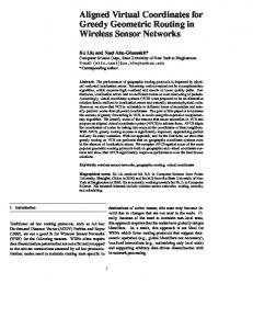
What is different in this paper is that we directly compute the map of the geometric domain R to a circular domain D. The shape of the domain R can be obtained through external sources such as a map and can be represented by a polygon. We will compute the mapping offline (on a centralized machine) and then use a small number of parameters to compactly represent the map. The number of parameters is the same as the complexity of describing the geometric domain R (e.g., the number of vertices of the polygon describing R), and is typically a small number in practice1 . Thus the parameters for the conformal map can be preloaded and programmed on the sensor nodes before deployment and each node can by itself calculate the virtual coordinates with its current geographical location. This representation is compact and stable. It does not depend on the network topology and does not change when the nodes move around. Besides the application in the mobile setting, the new method is also the first practical solution for applying virtual coordinates in a static sensor network. In the following we first report the theory and algorithms for computing and encoding the compact conformal map. Then we report results in our simulation and experiments. We implemented and tested the new method on a real testbed (the Orbit testbed [1]), a wireless network emulator with 400 nodes on a 20 by 20 grid. We compared routing using geographical locations and virtual coordinates, in both static and mobile network settings. Experimental results confirm that using the compact conformal map one can substantially improve the delivery rate and largely reduce the packet delay. II. BACKGROUND OF C ONFORMAL M APPING Given a domain R with an irregular shape and possibly holes, we would like to map it to a circular domain Ω, in which all boundaries are circular. To deform the domain, we are changing two measures, the metric that defines distances and the length of a curve, and the curvature, which describes how much a geometric object deviates from being flat in the case of a surface, or straight in the case of a curve. In our particular case, both R and Ω are flat, all points in the interior have zero curvature in both cases. But we need to change the curvature on all boundary points in R to be uniform (and thus being circular in Ω). Consider the simple case of deforming a simple polygon to a disk, as shown in Figure 1. For the boundary of a polygon, the points in the interior of boundary edges have curvature zero; and the vertices have non-zero curvature, defined as the turning angles at this vertex between the two adjacent edges. To make the curvatures at all these vertices the same (thus the polygon being regular) we need to change the metric as well, i.e., stretching the polygon in certain ways. The tool to compute the deformation is Ricci flow. In particular, Ricci flow deforms the Riemannian metric proportional to the local curvature, such that the curvature evolves according to the heat diffusion process. Eventually, curvature 1 There are numerous work on the simplification and approximation of a polygon [7]. By allowing reasonable approximation one can substantially reduce the complexity of a polygon.

at all points converge and the surface has uniform curvature. In order to deform a surface to be a particular shape, we can specify the target curvature and define Ricci flow by deforming the metric according to the difference of the local curvature and the target curvature. When Ricci flow converges we get the shape with the target curvature. In our case we will specify Ω such that all points in the interior have zero curvature and points on the same (interior/outer) boundary have uniform (negative/positive) curvature. Ricci flow has been applied in the proof of Poincar´e conjecture by Perelman in [22]. In the current work, we apply surface Ricci flow theory developed by Hamilton [14] and Chow [6]. The earlier work by Sarkar et al. [24] developed the distributed algorithm for implementing Ricci flow in a static sensor network. The process of Ricci flow defines a map from the original surface R to the deformed surface Ω. This map is conformal. A conformal map between two surfaces preserves angles. For any two arbitrary curves γ1 , γ2 on the surface S, a conformal map ϕ maps them to ϕ(γ1 ), ϕ(γ2 ) with the same intersection angle as that of γ1 , γ2 on S. In our application we assume that a set of wireless sensor nodes densely cover the domain R, which is represented by a polygon with possibly inner holes. In this paper we show that the the conformal mapping f from R to a circular domain can be encoded by a small number of parameters — the number of these parameters is the same as the complexity of describing R and in practice is small. These parameters are preloaded to all the sensors in the network such that each sensor can compute the virtual coordinates, i.e., coordinates under the mapping f by itself. The two sections below describe the encoding of f and the algorithm to compute the virtual coordinates with the encoded map respectively. III. S CHWARZ -C HRISTOFFEL T RANSFORMATION U SING L AURENT S ERIES To encode a conformal map, we introduce the SchwarzChristoffel formula and the Laurent series [8], [10], for simply connected domains (i.e., domains without holes) and multiply connected domains (i.e., domains with holes), respectively. A. Simply Connected Domain 𝑧5

𝑤5 𝑧4

𝑧6

𝛽4𝜋

𝑤4

𝑓 𝑤6

𝑤8 𝑤7

𝛽8𝜋

𝛽6𝜋

𝛽7𝜋

𝛽3𝜋 𝑤3

𝑧3 𝑧7 𝛽2𝜋 𝑧8

𝑧2

𝑤1

𝛽1𝜋

𝑤2

𝑧1 𝑧 − 𝑝𝑙𝑎𝑛𝑒

𝑤 − 𝑝𝑙𝑎𝑛𝑒

Fig. 1. The Schwarz-Christoffel transformation for a simply connected domain. f (zi ) = wi .

In the case of sensors in a simply connected domain R, as shown in Figure 1, we would like to find a mapping to a

unit disk D. We first look at the conformal mapping from the unit disk to a polygon R, which is a holomorphic function2 , f : D → R. The mapping we would like to encode is the inverse of f , f −1 : R → D. Suppose the vertices of the polygon are {w1 , w2 , · · · , wn }. The Schwarz-Christoffel formula [10] describes the mapping of a disk onto the interior of a simple polygon. ∫ z∏ n f (z) = A (ζ − zk )−βk dζ + B, (1) k=1

where the pre-image of wk on the circle is zk , i.e., wk = f (zk ); the polygon tangent turning angle at wk is βk π; A and B are two constants. In our case, we need to compute the inverse f −1 : R → D. For convenience, we denote g(w) = f −1 (w). Suppose w0 = f (0). For each w ∈ R, we choose a path connecting w0 and w, then ∫ w dg(w) −1 g(w) = f (w) = dw + 0. dw w0 where the derivative is given by ( )−1 ∏ n n ∏ dg(w) df (z) = = (z − zk )βk = (g(w) − zk )βk . dw dz k=1

k=1

Therefore we can calculate g(w) as: ∫ w∏ n g(w) = (g(τ ) − zk )βk dτ + 0.

(2)

w0 k=1

This is a typical ODE (ordinary differential equation) problem, and can be easily solved by Runge-Kutta method [5]. Therefore, each sensor only requires the parameters {zk , βk }nk=1 and the constants A, B. With such information every sensor can solve the ODE and obtains its own location. The number of parameters stored on each sensors is linear in the complexity to describe R. If we approximate R with simpler polygon we can reduce the storage requirement accordingly. The evaluation of the conformal map is equivalent to performing a path integration, the shorter the path is, the faster the evaluation is. Therefore in the mobile network setting we can update the virtual coordinates of a mobile node based on its current location, the past location and the past virtual coordinates. This will be faster than direct computation. Suppose at the j-th step, a node’s position is w(j) , its virtual coordinates is z (j) . Then at the k + 1-th step, if the position is w(j+1) , the virtual coordinate z (j+1) can be updated as ∫ (j) z = f ′ (ζ)dζ, γ

where γ is the path connecting w(j) to w(j+1) . B. Multiply Connected Domain The formulation for conformal mappings for multiply connected domains is very similar. Recall that by using Ricci flow 2 A holomorphic function is a complex-valued function of one or more complex variables that is complex differentiable in a neighborhood of every point in its domain.

𝑧2,2 𝐶2

Ω

Γ2

𝑃

𝐶1 𝑧3,2 𝑧2,1 𝑐1 𝑟1 𝑧1,1

𝑧1,2

𝑤3,1 Γ1 𝑓

𝐶3

𝑤1,2 𝑤2,1

the following formula, called the Laurent series: βk,j  ∫ f (z) = A

𝑤4,1

𝑤1,1 Γ3

Fig. 2. The Schwarz-Christoffel transformation for a multiply connected domain. f (zi,j ) = wi,j .

on the polygon R (with m−1 holes) describing the domain of interest, we map it to a circular domain Ω with m − 1 circular interior holes. Now we apply a reflection on Ω to make it an unbounded domain with m circular holes. A reflection through a circle maps the interior of the circle to the exterior. Suppose p is a point inside the circle Cj (cj , rj ), then it is reflected to q, where p − cj 2 q= r + cj |p − cj |2 j In particular, we can reflect the circular domain Ω with respect to the outer boundary and project it to an unbounded domain with m circular holes. This extra reflection is also conformal. For the ease of description, we will assume from now on that Ω is an unbounded domain with m circular holes. Similar to the simply connected case, there is a description of a conformal mapping f from an unbounded domain Ω with m circular holes to an unbounded domain R with m polygonal holes. Again what we want to use is the inverse of f , say g = f −1 . As shown in Figure 2, let Cj be the j-th circular hole, with center cj and radius rj , which is mapped to a polygonal hole Γj , f (Cj ) = Γj . The vertices of Γj are {w1,j , w2,j , · · · , wkj ,j } ⊂ Γj . Their pre-images are {z1,j , z2,j , · · · , zkj ,j } ⊂ Cj .

Fig. 3. Circle reflection.

On the circular domain Ω we will apply reflections with respect to the circles. As shown in Figure 3, a circle Cj is reflected through circle Ci to get a circle Cij . A circle Ck is reflected through the circle Cij to get a circle Cijk . More generally, a circle Cin is reflected through the circle Ci1 i2 ,···in−1 to get Ci1 i2 ,··· ,in . The multi-index i1 i2 , · · · , in tracks the sequence of reflections. The set of all multi-indices with length n is denoted as σn . The conformal mapping f : Ω → R can be computed using

 ( ) ∞  ∏ ζ − zk,νj       ζ − sνj  j=1 k=1   n=0 ν ∈ σn

Kj m ∏ z ∏

dζ + B.

(3) where zk,νj are reflections through circles of prevertices zk,j ; sνj are reflections of circle centers sj = cj ; ν is a multi-index tracking reflections; A and B are two constants. Similar to the simply connected domain case, the inverse of f can be evaluated by solving an ODE. In practice, instead of using infinitely many reflections, one can reflect only N times, for a reasonable N . In practice N is less than 5. Therefore, the Laurent series could be approximated by:  βk,j ∫ f (z) = A

 ( ) N  ∏ ζ − zk,νj        ζ − s νj j=1 k=1   n=0 ν ∈ σn

Kj m ∏ z ∏

dζ + B.

(4) In the formula, the prevertices {zk,j } and the circle domain Cj (cj , rj ) are computed using the Ricci flow method offline, say by using the method in [24]. Then these values are preloaded to all the sensors with the tangent turning angle {βk,j } and the constants A, B. Each sensor’s virtual coordiantes can be computed through the conformal mapping f −1 : P → Ω by solving an ODE. IV. E XAMPLES In this section, we elaborate the computation of the virtual coordinates using specific examples. These two examples are what we used in the following experiments.

(a) Vertices of R

(b) mapped to a circle

Fig. 4. Conformal map from a circle to R using Schwartz-Christoffel formula.

A. Simply Connected Domain Suppose the sensors move within a simply connected domain as shown in Figure 4(a). A conformal map f maps a unit disk as shown in Figure 4(b) to R such that f (zi ) = wi , where wi are vertices of R. Table I shows the coefficients for the Schwarz-Christoffel transformation, where w are the coordinates of the polygon vertices, z are the prevertices on the

w 1 + 1i 20 + 1i 20 + 8i 5 + 8i 5 + 13i 20 + 13i 20 + 20i 1 + 20i

β 0.5 0.5 0.5 -0.5 -0.5 0.5 0.5 0.5

A B

z -0.98993 + 0.14155i -0.99478 + 0.10202i -0.99480 + 0.10184i -0.99978 - 0.02078i 0.97883 - 0.20466i 0.99872 - 0.05063i 0.99873 - 0.05041i 1.00000 + 0.00000i

-0.16623648 + 2.5343952i 3.15 + 10.65i

Note: w - polygon domain, z - disk domain, βπ - tangential turning angle, A - constant scalar in transformation, B - conformal center on w. TABLE I. Parameters of Schwarz-Christoffel transformation.

unit disk domain, A is a constant scalar, B is the conformal center which is mapped to the origin of the unit disk, β is the tangential turning angle of the input polygon boundary. The prevertices for the interior sensors can be computed by Equation 2 using the obtained coefficients above. B. Multiply Connected Domain Suppose the mobile sensors move within a multiply connected domain as shown in Figure 5 (a). We first use Ricci flow to conformally map the domain to a circle domain, as shown in Figure 5(b). Through this initial mapping, we obtain the coefficients in Equation 4, as shown in Table II. The prevertices for the interior sensors can be evaluated by solving an ODE to compute the inverse function of Equation 4 with the obtained coefficients. A

B

(a) Input domain R.

(b) Mapped to a circular domain.

Fig. 5. Ricci flow for conformal mapping a multiply connected polygon.

V. E XPERIMENTAL R ESULTS In this section, we compare the proposed virtual-coordinate based greedy routing with the traditional greedy routing based on the original geographical locations, and NoGeo routing proposed by Rao et al. [23] in both static and mobile network settings. In NoGeo, a set of virtual coordinates are computed by fixing the network outer boundary at a square box and running iterative computations to put each non-boundary node at the center of mass of its neighbors until convergence. We did not implement any recovery scheme (e.g., face routing [16]) when greedy routing (based on whatever coordinates) fails at a local minimum. The reasons for such consideration are the following: first, such recovery schemes are more complicated and are usually developed for an idealistic setting; second, for mobile networks it makes less sense to try to recover

w 0 30 + 1i 30 + 30i 30i 4 + 15i 4 + 26i 14 + 26i 14 + 22i 7 + 22i 7 + 19i 14 + 19i 14 + 15i 13 + 4i 13 + 8i 22 + 8i 22 + 16i 26 + 16i 26 + 4i

β 0.5 0.5 0.5 0.5 -0.5 -0.5 -0.5 -0.5 0.5 0.5 -0.5 -0.5 -0.5 -0.5 0.5 -0.5 -0.5 -0.5

(c1 , r1 ) (c2 , r2 ) A B

z -0.0769204 -0.997173i 0.994966 + 0.100535i 0.0887658 + 0.995941i -0.966776 + 0.256636i -0.592622 - 0.175069i -0.832789 + 0.236657i -0.482482 + 0.47661i -0.270788 + 0.371865i -0.246845 + 0.342856i -0.246771 + 0.342755i -0.226475 + 0.311561i -0.184719 + 0.109243i 0.479915 - 0.319252i 0.182277 - 0.133036i 0.138806 + 0.104056i 0.218467 + 0.283291i 0.494831 + 0.417102i 0.867876 + 0.0811398i

(-0.507853 + 0.159686 i, 0.327225) (0.513089 + 0.054973 i, 0.358639) -0.21564355 + 2.27355436i 16.45 + 11.65i

Note: w - polygon domain, z - circle domain, βπ - tangential turning angle, (ck , rk ) - center and radius of hole k on circle domain, A - constant scalar in transformation, B - conformal center on w. TABLE II. Parameters of Laurent series.

from local minimum as nodes move around and a packet may only get stuck temporarily; third, in our applications for participatory sensing and opportunistic query, it is not so critical that every message must be delivered – a scheme with sufficiently high success ratio that emphasizes on efficiency and low overhead will be more desirable. The experiments are performed by both computer simulations and real testbed emulations. The computer simulation is based on a computer generated network with 1000 nodes. The emulation is deployed on Orbit, an open accessed testbed [1]. We evaluated three performance metrics, namely, message delay (how long it takes to deliver a packet from source to destination; the number of hops (the number of nodes the packets visited when it is indeed delivered); and delivery rate (the fraction of successfully delivered packets). A. Simulation Results In the simulations, we considered both static and mobile networks. A

B

(a) mobile sensors

(b) virtual coordinates

Fig. 6. Mobile sensors at one snapshot.

t =0

t =2

t =3

t =4

t =5

t =6

t =7

t =8

t =32

t =65

Fig. 7. Greedy routing using real coordinates from the large red node (source) to the yellow node (destination). The green node on each frame shows the node holding the packet at time t. Greedy routing got stuck at time frame 8 and 32.

t =0

t =3

t =5

t =8

t =11

Fig. 8. Greedy routing using virtual coordinates for the same source destination pair as in Figure 7. A

Uniformly and randomly selected pairs Methods delivery rate hops Geographical locations 275/400 5.6 NoGeo 390/400 8.21 Our method 400/400 8.52 Specially chosen pairs Methods delivery rate hops Geographical locations 0/400 0 NoGeo 363/400 16.67 Our method 398/400 17.23 TABLE III. Simulation results on static networks.

B

(a) active nodes on orbit

(b) virtual coordinates

Fig. 9. Active nodes on orbit.

1) Experimental setup: We place 1000 nodes uniformly randomly inside a polygon with the boundary of [1,1], [20,1], [20,8], [5,8], [5,13], [20,13], [20,20], [1,20], as showed in Figure 6 (a). The communication links are generated by using the Unit Disk Graph (UDG) model with radius of 2. The average degree in the resulted communication graph is about 7. The corresponding domain under conformal mapping to a unit disk is shown in Figure 6 (b). All the results here are based on 400 pairs of delivery attempts, which are chosen in two different ways: 1) uniformly and randomly selected from the entire network; 2) uniformly randomly chosen from the special areas A and B in Figure 6 (a)

respectively, under which greedy routing based on geographical locations would have difficulty in delivering the packets, particularly in static setting. The 400 pairs are the same for the two algorithms for fairness. In the following we only reported the results for simply connected domain. The performance comparison for nonsimple domain is similar and thus omitted due to space constraint. 2) Static setting: In this setting nodes are stationary. We set TTL high enough such that packets can be delivered as long as there are valid routes. Thus, the only reason a packet could not be delivered is due to local minimum. The simulation results are shown in Table III. We can see from the results that the delivery rate of our method is much better than greedy routing with geographical

location, especially for the pairs in the specially chosen areas, for which greedy routing using geographical locations always gets stuck. We also have better delivery rate than NoGeo method. The number of hops listed in the table is the average value of hops for successfully delivered message. The hops for our method is higher than that of greedy routing with geographical locations, simply because our method can successfully deliver more messages, including the far apart pairs in the special area for which greedy routing using geographical locations fails. For the 275 pairs that could be delivered by greedy routing using geographical locations, the average number of hops using our method is only 5.88, only slightly higher than 5.6 using geographical locations. 3) Mobile setting: To evaluate our algorithm for the mobile setting, we adopt the popular Random Waypoint (RWP) mobility model [4]. Each node moves to a destination, uniformly randomly chosen in the domain R, along a straight line with fixed velocity. Upon arrival at the destination it stays for a period of time t (uniformly randomly drawn from [0, 2]), chooses the next destination and moves there along a line. The moving speed for node i is drawn from [0.5, 2.5] uniformly randomly. We sample the time axis to generate a sequence of snapshots, such that we only construct the communication neighbors and perform routing attempts at each snapshot. The sampling rate is uniformly distributed in the range [1, 3]. When the node with the packet is within transmission range of the destination location, the packet is considered delivered successfully. If the package gets stuck, it remains at the current node for another trial in the next time slot. Notice that in the next snapshot, the node with the packet moves to a different location and may have a new set of neighbors. See Figure 7 and Figure 8 for examples. We use TTL to control how long the packets could wander in the network. When a packet is delivered, we measure the delay as the number of snapshots experienced when the packet arrives at the destination. We measure the number of hops of a successfully delivered packet as the number of relay nodes on the path from its source to the destination. The results are concluded in Table IV. We can observe from the results that the delivery rate is substantially improved when mobility is allowed, both for greedy routing using geographical locations, NoGeo method and our method. Nevertheless we could deliver the messages with much smaller delay and hops. In particular, notice that in our experiments the values for hops and delay are always the same for our method. This means our method never gets stuck — in every time slot we are able to find a neighbor that is closer to the destination; the message is never held at a node for more than one time unit. This explains the reduced delay and the high delivery rate. For the messages that are indeed delivered within small TTL in greedy routing method using geographical locations, the delay and hop counts experienced are similar to that in our methods. When the TTL is large, the pairs delivered under geographical locations method have more hops and delay compared to our method. This basically says that for messages that start at positions whose straight line paths to the destination are not ‘blocked’, and they can

Geographical locations method on uniformly randomly chosen pairs TTL delivery rate hops delay 10 238/400 5.15 5.15 20 286/400 6.28 6.29 30 295/400 6.69 6.76 200 338/400 17.39 19.36 Geographical locations method on specially chosen pairs TTL delivery rate hops delay 10 0/400 0 0 20 1/400 18 19 30 2/400 22.5 23.5 200 173/400 95.62 110.8 Our method on randomly chosen pairs TTL delivery rate hops delay 10 231/400 5.28 5.28 20 379/400 8.43 8.43 30 400/400 9.12 9.12 Our method on specially chosen pairs TTL delivery rate hops delay 10 0 0 0 20 254/400 16.50 16.50 30 400/400 18.40 18.40

Our method on delivered pairs under geographical locations delivery rate hops delay 215/238 5.02 5.02 286/286 6.58 6.58 295/295 6.79 6.79 338/338 7.95 7.95 Our method on delivered pairs under geographical locations delivery rate hops delay 0/0 0 0 1/1 18 18 2/2 19 19 173/173 19.02 19.02 NoGeo method on randomly chosen pairs delivery rate hops delay 220/400 5.13 5.13 382/400 8.68 8.68 400/400 9.22 9.22 NoGeo method on specially chosen pairs delivery rate hops delay 0 0 0 248/400 16.67 16.69 399/400 18.43 18.46

TABLE IV. Performance of the methods under mobile setting of computer simulation.

be delivered fairly quickly and easily, using both methods. But for messages that get stuck, using geographical locations they will need to wait for a long time for the node holding them to move out of that region; using our methods they have no problem to find good neighbors. Although in terms of delivery rate our method and NoGeo method are comparable, the computational cost under NoGeo is far heavier than ours. Under our method, for each TTL the virtual coordinate for each node is obtained locally using a small number of pre-calculated parameters; while in NoGeo one needs to recompute the virtual coordinates for around 160 iterations. Note that, if we aim for lower computational cost, say, updating the coordinates every 5 TTL under NoGeo, the delivery performance is not as good as the results we show in Table IV, with delivery rate as 246/300 for special chosen pairs. Thus our method has superior delay and cost tradeoffs. B. Emulation on Orbit In this section, we demonstrate results from emulation experiments on a real testbed to validate our algorithm and compare to greedy routing with geographical locations. The emulation is deployed on the publicly accessible Orbit testbed [1]. This testbed consists of 400 nodes (standard Linux PCs), and it supports both wired and wireless experiments. The nodes are placed in a two-dimensional rectangular grid with 1 meter spacing and wireless antennas mounted on the sides. 1) Experimental setup: The network we created on Orbit has the same boundary as what we used in the simulations. There are 340 nodes in this C-shape area. Among them 233 nodes (shown in Figure 9 (a)) of the grid are active nodes on Orbit. The rest nodes are artificially removed from our experiments. In our experiments, not all nodes selected are

available to use and nodes may go down for no reason. So we do not have uniformly distributed nodes per our observation. The corresponding map of the network and virtual coordinates is shown in Figure 9 (b). The network topology is created with a unit disk graph model with communication range of 2.5. For two nodes within communication range, we use the wired communication channel on Orbit for packet transmission in the experiments, since the wireless radios on Orbit were set up with very large communication range, essentially covering the entire network. UDP is chosen as the communication protocol between the nodes. Although the communication graph is selected from a unit disk graph model, the packet is not always delivered even if the sender and receiver are within transmission range. This is observed from our experiments and could be observed from the results reported later. Each of the node is equipped with two functions. 1) Initialize a packet as the sender and send it to the next node. 2) Listen and forward the message to the next node. The two functions are designed as threads, so the nodes can have the two functions at the same time. This simulates the scenario of a node in full duplex mode. We utilized a link table to filter packets at the application layer so that each node only receives the messages from its neighbors within communication range. Since the local clocks at the Orbit nodes are not consistent, we cannot directly take the difference of the packet departure and arrival time. Instead, we work around this issue by sending a confirmation from the destination back to the source. Therefore the delay reported in our result actually includes this extra ‘acknowledgement’ step. Notice that since this extra step is added to both methods the comparison is still fair. The value for delay reported later is the median value. 2) Static setting: 40 pairs of source and destination are chosen among the above 233 nodes for routing. The nodes’ geographical coordinates are their grid coordinates. Same as in computer simulation, the pairs are uniformly randomly chosen and chosen from area A and B in Figure 9 respectively in two different ways. Each node can obtain the locations of other nodes from the global node location table. And nodes can get their neighbor information from the global link table. To run our experiments, we issue 40 pairs of packets through the central controller. The sender initializes a packet with destination information and sends it to one of the neighbors according to the greedy algorithm. Since all the nodes listen in the network. If a packet is sent to a node, the node catches it. The node will then forward the packet to the next node until the packet arrives at the destination. The choice of which neighbor to send packet to depends on the node’s location and connection specified in the global node locations table and global link table. The experiment setups for both greedy routing with geographical coordinates and virtual coordinates are the same except the different set of coordinates. We compare delay, hops and delivery rate under the two methods, with randomly chosen pairs and specially chosen pairs. The results are listed in Table V.

Uniformly randomly chosen pairs Methods delivery rate hops Geographical locations 27/40 5.8 Virtual coordinates 40/40 8.23 Specially chosen pairs Methods delivery rate hops Geographical locations 0/40 0 Virtual coordinates 38/40 16

delay (ms) 25.669 29.631 delay (ms) 0 33.270

TABLE V. Performance of the methods under static setting of Orbit emulation.

We simulate the experiment with all the same setting on the computer, and the delivery rate for virtual coordinates routing under special chosen area is 40/40. Notice that some of the delivery rate under our simulations (the ideal setting) is higher than the results we get from Orbit experiments. The reasons are 1) the Orbit network may experience unknown stability issues and packets may get lost for no reason (since UDP is used); 2) two packets may arrive at a node at the same time. Thus due to competition (similar to wireless interference) one of them may be lost; 3) the nodes may be go up and down during the experiments Nevertheless this represents a practical setting in which transmission failures may as well occur. Under the same network condition, our method consistently works better than greedy routing with geographical locations, especially for pairs in the special chosen areas. The results are similar to the results obtained in our computer simulations. 3) Mobile setting: The nodes on Orbit are static. In order to mimic a mobile network on Orbit, we generate a mobile network scenario using simulations and then map the mobile nodes in our simulations onto the Orbit nodes. A mobile node is mapped to the closest Orbit node. In this case, we can use the movement of nodes from computer simulation to emulate the mobility of nodes on Orbit. Thus, the nodes move in the same way as reported earlier and the actual transmission are done on Orbit. 40 pairs of packets are chosen randomly uniformly and from the special area same as the above experiments respectively. Different from computer simulation, the delay on real testbed of Orbit is the real time difference between the message sent and received. The results are reported in Table VI. The observation that mobility helps to improve delivery rate still holds for the testbed experiments, for both geographical greedy routing and our method. Again our method gives much smaller delay and fewer number of hops. We may notice that there could be a large deviation from the hop counts and packet delay, in particular for geographical greedy routing for specially selected pairs. As in geographical greedy routing, many packets go through some small number of critical nodes. In our simulations we assume that all these packets go through with ease – an unrealistically ideal case. But on Orbit, when an Orbit node is called by several packets (invoked frequently), a queue is formed and this could substantially increase the delay. VI. C ONCLUSION This paper describes a compact way to represent a conformal map and applies it to routing in both static and mobile

Greedy routing using geographical locations on uniformly randomly chosen pairs TTL delivery rate hops delay (ms) 10 21/40 5.20 31.215 20 24/40 6.12 32.275 30 25/40 6.71 33.130 200 29/40 10.56 43.873 Greedy routing using geographical locations on specially chosen pairs TTL delivery rate hops delay (ms) 10 0/40 0 0 20 0/40 0 0 30 1/40 12 93.978 200 10/40 50.72 629.985 Greedy routing using virtual coordinates on uniformly randomly chosen pairs TTL delivery rate hops delay (ms) 10 21/40 5.22 31.582 20 33/40 8.27 32.232 30 37/40 9.01 32.775 Greedy routing using virtual coordinates on specially chosen pairs TTL delivery rate hops delay (ms) 10 0/40 0 0 20 21/40 14.28 52.536 30 32/40 16.21 71.700 TABLE VI. Performance of the methods under mobile setting of Orbit.

networks. As the first practical solution to using virtual coordinates with greedy routing, we expect to see implementations of our method in real world applications. ACKNOWLEDGMENT The authors would like to acknowledge the support from NSF through DMS-1221339 and CNS-1016829. R EFERENCES [1] Orbit testbed. http://www.orbit-lab.org/. [2] P. Angelini, F. Frati, and L. Grilli. An algorithm to construct greedy drawings of triangulations. In Proc. of the 16th International Symposium on Graph Drawing, pages 26–37, 2008. [3] P. Bose, P. Morin, I. Stojmenovic, and J. Urrutia. Routing with guaranteed delivery in ad hoc wireless networks. Wireless Networks, 7(6):609–616, 2001. [4] J. Broch, D. A. Maltz, D. B. Johnson, Y.-C. Hu, and J. Jetcheva. A performance comparison of multi-hop wireless ad hoc network routing protocols. In Proc. of the ACM/IEEE Mobile Computing and Networking (MobiCom), pages 85–97, 1998. [5] J. C. Butcher. Numerical Methods for Ordinary Differential Equations. New York: John Wiley & Sons, 2002. [6] B. Chow. The ricci flow on the 2-sphere. J. Differential Geom., 33(2):325–334, 1991. [7] M. de Berg, M. van Kreveld, M. Overmars, and O. Schwarzkopf. Computational Geometry: Algorithms and Applications. Springer-Verlag, Berlin, 1997. [8] T. DeLillo and E. Kropf. Numerical computation of the schwarzchristoffel transformation for multiply connected domains. SIAM J. on Scientific Computing, 33:1369–1394, 2011. [9] R. Dhandapani. Greedy drawings of triangulations. In SODA ’08: Proceedings of the nineteenth annual ACM-SIAM symposium on Discrete algorithms, pages 102–111, 2008. [10] T. A. Driscoll and L. N. Trefethen. Schwarz-Christoffel Mapping, volume 8. Cambridge University Press, 2002. [11] D. Eppstein and M. T. Goodrich. Succinct greedy graph drawing in the hyperbolic plane. In Proc. of the 16th International Symposium on Graph Drawing, pages 14–25, 2008. [12] R. Flury, S. Pemmaraju, and R. Wattenhofer. Greedy routing with bounded stretch. In Proc. of the 28th Annual IEEE Conference on Computer Communications (INFOCOM), April 2009.

[13] M. Grossglauser and D. Tse. Mobility increases the capacity of ad hoc wireless networks. IEEE/ACM Transactions on Networking, 10(4):477– 486, August 2002. [14] R. S. Hamilton. Three manifolds with positive ricci curvature. Journal of Differential Geometry., 17:255–306, 1982. [15] X. He and H. Zhang. On succinct convex greedy drawing of 3-connected plane graphs. In Proceedings of the ACM-SIAM symposium on Discrete algorithms, pages 1477–1486, January 2011. [16] B. Karp and H. Kung. GPSR: Greedy perimeter stateless routing for wireless networks. In Proc. of the ACM/IEEE International Conference on Mobile Computing and Networking, pages 243–254, 2000. [17] Y.-J. Kim, R. Govindan, B. Karp, and S. Shenker. On the pitfalls of geographic face routing. In DIALM-POMC ’05: Proceedings of the 2005 joint workshop on Foundations of mobile computing, pages 34–43, 2005. [18] R. Kleinberg. Geographic routing using hyperbolic space. In Proceedings of the 26th Conference of the IEEE Communications Society (INFOCOM’07), pages 1902–1909, 2007. [19] T. Leighton and A. Moitra. Some results on greedy embeddings in metric spaces. In Proc. of the 49th IEEE Annual Symposium on Foundations of Computer Science, pages 337–346, October 2008. [20] P. Maymounkov. Greedy embeddings, trees, and euclidean vs. lobachevsky geometry. manuscript, 2006. [21] C. H. Papadimitriou and D. Ratajczak. On a conjecture related to geometric routing. Theor. Comput. Sci., 344(1):3–14, 2005. [22] G. Perelman. The entropy formula for the ricci flow and its geometric applications. Technical Report arXiv.org, November 11 2002. [23] A. Rao, C. Papadimitriou, S. Shenker, and I. Stoica. Geographic routing without location information. In Proceedings of the international conference on Mobile computing and networking, pages 96–108, 2003. [24] R. Sarkar, X. Yin, J. Gao, F. Luo, and X. D. Gu. Greedy routing with guaranteed delivery using ricci flows. In Proc. of the 8th International Symposium on Information Processing in Sensor Networks (IPSN’09), pages 97–108, April 2009. [25] K. Seada, A. Helmy, and R. Govindan. On the effect of localization errors on geographic face routing in sensor networks. In IPSN ’04: Proceedings of the third international symposium on Information processing in sensor networks, pages 71–80, 2004.