Based on recent experimental hints we hypothesize that brain, for effective representation of time-evolving .... The agent is free to chose among different alternatives, e.g., by ...... Bear, M.F.; Conners, B.W. & Paradiso, M.A. (2007). Neuroscience: exploring the brain. Williams. & Wilkins. 3rd Ed. Cruse, H. ... McGraw-Hill, 4th ed.
6 Compact Internal Representation as a Functional Basis for Protocognitive Exploration of Dynamic Environments Valeri A. Makarov and José Antonio Villacorta-Atienza Universidad Complutense de Madrid Spain
1. Introduction Nature has provided living beings with a set of cognitive properties that enables subjective perception of the external world with the aim of constructing behaviors and survival within specific environments. A simple but comprehensive example is a near-range searching for a target by a mobile agent in a time-evolving environment. It requires fast and reliable generation of flexible behaviors that must take into account not only the current state of the environment and of the agent, but also infer on their future states. Despite a vast literature and numerous contexts where the concept of cognition appears [see, e.g., (Baars & Gage, 2010; Newell, 1994; Wasserman & Zentall, 2009)], there is no generally accepted functional definition. Nevertheless capacities such as Internal Representation (IR) of the external world, memory, and learning are commonly accepted as elements constituting cognition (Godfrey-Smith, 2001). For the study of the problem of cognitive exploration of dynamic environments it seems sensible to restrict the cognitive abilities to those manifested externally in motricity, i.e. to those experimentally verifiable in animal models. Then we can speak about “initial stages” of cognition or protocognition, a subject that has been for decades a hot spot both in theoretical and experimental (mainly in insects and mammals) research [see, e.g., (Cruse, 2003; Hesslow, 2002; Newell, 1994) and references therein]. In this chapter as a working hypothesis we use a general functional definition of protocognition as the basis levels of the “Cognitive Pyramid” given by Wray et al. (2007). Namely, the protocognitive capacities organize the sensory information into structured representations, which provide “skeletal subsolutions” for the higher cognitive levels. The complexity of protocognitive skills stems from several factors shared by living beings. First, an enormous amount of sensory information must be structured and broken into aspects relevant for the aim-driven perception (e.g., position and shape of a target), while discarding the rest. Usually this is done by the agent’s sensory system, which provides highly specialized information to the central nervous system (Bear et al., 2007; Kandel et al., 2000). Second, a serious source of complexity is the continuous evolution of the environment and causal relations among its constituents. This requires anticipation and hence a predictive model of the environment and of the agent itself. The cognitive neuronal pathways or circuits are in charge of building up forward world models based on genetic wiring and experience. Then the external input modulates the (nonlinear) dynamics of the neuronal
82
Neural Networks for Temporal Data Processing
circuits, which produce behaviors ready to be selected by upper cognitive levels (e.g., using motivation) and to be enacted. Third, an efficient (fast, reliable, and flexible) management of behavioral problems relies on memorization of novel situations and learning associations with corresponding successful behaviors. Libraries of stereotypic situations can significantly speedup the agent’s reaction and make automatic the previously learned behaviors converting them into subconscious states. An example is an experiment with astronauts catching a ball under reduced effective gravity (McIntyre et al., 2001). At the beginning of the experiment the peak of anticipatory muscle activation occurred earlier than the real impact of the ball, which lead to incorrect, biased by the experience in the Earth, behaviors. However, after a few days the astronauts adapted to the new conditions, i.e. the inner mental “model of the ball trajectory” successfully learned new parameters and finally were able to “calculate” reliably and fast the necessary movement. It is noteworthy that the first two features set the ground level of the Cognitive Pyramid, whereas the third one belongs to the intermediate floor and operates over the information provided by the ground level. Then intriguing questions are: what are the basic principles of organization and operation of the cognitive pathways? and how can we mimic them? An answer to these questions, besides its theoretical value, also would enable a qualitative advance in mobile robotics. Here we develop a paradigm of protocognitive neuronal pathways involved into exploration of dynamic environments based on the so-called principle of Compact Internal Representations (CIRs) of interactions between the agent and its environment (Villacorta-Atienza et al., 2010). Based on recent experimental hints we hypothesize that brain, for effective representation of time-evolving situations, may use specific time-space transformation that reduces the corresponding time-dependent structures into static patterns that can be easily compared, stored, and organized into “libraries”. Then the protocognitive pathways should include several basic elements: i) Preliminary sensory blocks, capable of extracting the information essential for prediction of the future states of the environment; ii) A substrate responsible for the IR, which models a set of virtual futures induced by agent’s decisions (e.g., collisions with obstacles in the time-space domain); iii) Working memory that is used for learning and storing the previous successful experiences, which can optimize and speedup the decision making. In Sect. 2 we show how the modeling of time-space collisions can be implemented in a two-dimensional (2D) neuronal network. The network, called Causal Neural Network (CNN), exploits in a mental world model the principle of causality, which enables reduction of the time-dependent structure of real dynamic situations to compact static patterns. A single point in the multidimensional phase space of the CNN gives a CIR of the dynamic situation. Such CIR provides complete description of the time-space collisions. A remarkable feature of CIRs is that they do not merely represent situations in which the agent is involved, but contain a set of behaviors adapted to these specific situations. These behaviors can be used as a basic entities in higher cognitive activity to create new solutions. In consequence CIR may be considered as a functional basis for protocognition. In Sect. 3 we study how individual memory items can be stored assuming that situations given in the environment can be represented in the form of synaptic-like couplings in a Recurrent Neural Network (RNN). We provide theoretical analysis illustrating the learning process and response to novel or incomplete stimuli and show that RNN is suitable for
Compact Internal Representation as a Functional Basis for Protocognitive Exploration of Dynamic Environments
83
simulation of working memory. Furthermore, we show that a similar RNN can be specially trained to perform algebraic operations over the input stimuli. This ability is essential for prediction of trajectories of moving objects, i.e. for modeling of future states of the environment. In Sect. 4 we provide a general architecture of a protocognitive agent, which includes conscious and subconscious pathways builded up on the basis of the neuronal networks discussed in Sects. 2 and 3. Then we illustrate generation of behaviors and their learning by the agent moving in realistic time-evolving environments. Special attention is given to dynamical construction of libraries of stereotypic situations and associated CIRs. We show how, based on the initial sensory information only, the agent can retrieve an appropriate CIR from the library and hence make fast and efficient decision. Finally in Sect. 5 we summarize our results.
2. Compact internal representation of complex environments static obstacle
Causal Neural Network
target
? y x
agent
moving obstacle
j i
Generation of CIRs
Fig. 1. Sketch of an arena containing an agent, a target, and static and moving obstacles. The agent perceives all objects in the arena and makes a decision on how to reach the target avoiding collisions with the obstacles. The decision making is based on Compact Internal Representations (CIRs) of itself and of the environment created in the Causal Neural Network. Internal Representation is a task-oriented inner description of the environment and of the agent itself, which offers distinct modes to fulfill a task. In what follows we discuss one specific decision making problem: a search for paths to a target by a mobile agent in a time-evolving environment (Fig. 1). For the sake of simplicity the target is considered immobile and can be an object or a specific place or even an area in the arena. We assume that the target and obstacles emit or reflect a signal, e.g., sound or light, which is perceived by the agent’s sensory system, and hence the agent can make a non-blind decision. To avoid obstacles (especially moving) the agent may construct a spatiotemporal IR of the observed dynamic situation and use it as a “world model” to resolve collisions. Such time-dependent IR should be based on prediction of the possible positions of the obstacles and of the agent in the (mental) future. However, time-dependent IRs due to their excessive complexity are not suitable for protocognitive behavior. A big challenge is to understand how the brain makes compact and efficient descriptions of time-evolving situations. In this section we describe an approach that enables reduction of time-dependent IRs to CIRs, i.e. to static patterns (Villacorta-Atienza et al., 2010). These static patterns emerge in the so-called Causal Neural Network (CNN), whose dynamics is driven by the sensory information (Fig. 1). Geometrically the CNN is an (n × m)-lattice of locally coupled neurons. The lattice coordinates (i, j) scale to real coordinates ( x, y) in the arena.
84
Neural Networks for Temporal Data Processing
2.1 Static environments
Let us first briefly describe how CIR can be created in the simplest case when all elements in a 2D arena (except the agent) are immobile. Then the sensory output is time independent, and hence the immobile obstacles and the target can be simply mapped into the corresponding cells in the CNN. The CNN models the process of virtual (mental) exploration of the environment by the agent. Conceptually, a number of identical virtual agents are released at the agent’s initial position (orange cell in Fig. 1) and perform a random search in the lattice space until they explore completely the “arena” or some of them reach the target’s image in the CNN. Then the distribution of the virtual agents in the CNN lattice defines the CIR, which further can be used for path planing. The dynamics of the CNN (for static environment) is given by: r˙ ij = dΔrij − rij pij
(1)
where rij is the neuronal state variable, representing the concentration of virtual agents at the cell (i, j); the time derivative is taken with respect to the mental (inner) time τ; Δrij = ri+1,j + ri−1,j + ri,j+1 + ri,j−1 − 4rij denotes the discrete Laplace operator describing the local (nearest neighbor) interneuronal couplings, whose strength is controlled by d; and pij accounts for the target: � 1, if (i, j) is occupied by target pij = (2) 0, otherwise It is worth pointing out that a target is not a real entity existing in the environment (as an object or place), instead it is designated by the agent’s motivation layer. For example, a football player can turn aside from or catch a ball depending on which side he plays on. Thus the target is not an external constraint but an internal emergent property of the brain, whose influence we model by the reactive term in (1). This differs from other approaches that postulate targets as singular elements in the environment [see, e.g., (Schmidt & Azarm, 1992)]. Obstacles are external constraints whose biological identity, provided by boundary cells (Savelli et al., 2008), suggests that they shape the IR through altering states of the neurons corresponding to the obstacle boundaries. We assume that the obstacles are solid non-penetrable objects, hence a virtual agent reaching an obstacle frontier rebounds and continues exploring the arena. Thus we impose zero-flux (Neumann) boundary conditions at the obstacle’s frontiers and also at the arena boundary. At τ = 0 no virtual agent exists, hence we set rij (0) = 0 for all CNN cells except those occupied by the agent, where rij (τ ) = ra for τ ≥ 0. It has been shown that stable steady states are the only attractors in the phase space Ψ = R nm + of the CNN (Villacorta-Atienza et al., 2010). Thus any trajectory in Ψ defined by initial conditions (except a null set) tends to one of the stable steady states {rij∗ } ∈ Ψ, which is the CIR of the given static situation. By unfolding this steady state into the three-dimensional lattice space {Z2 , R + } we get a 2D stationary pattern that can be used to trace paths starting at the agent location and crossing the contour lines. We note that rij∗ satisfies the discrete Laplace equation, and consequently the created pattern has no local minimums (Keymeulen & Decuyper, 1994; Louste & Liegeois, 2000). This ensures that all paths (except a null set) derived from this approach end at the target, and hence we obtain multiple alternatives to reach the target. To illustrate the approach we simulated a 2D arena consisting of an agent, two immobile obstacles, and a target (Fig. 2, left). The corresponding sensory information has been used to integrate numerically the CNN model. Figure 2 (right) shows the limit pattern {rij∗ }
Compact Internal Representation as a Functional Basis for Protocognitive Exploration of Dynamic Environments sensory information
85
CNN
Agent
Obstacles
Target
Fig. 2. Compact Internal Representation of static environments. Left panel: 2D arena consisting of an agent (red triangle), immobile obstacles (blue rectangles), and a target (green circle). Positions of all objects are mapped into the CNN whose relaxation yields a CIR, i.e. a ∗ static 2D pattern {rij∗ }60 i,j =1 . Right panel: Contour plot of {r ij } (colored curves from red to cyan). A set of paths start at the agent’s position and descend down the gradient to the target (blue arrowed curves). The agent is free to chose among different alternatives, e.g., by minimizing the path length (solid thick curve) or by rising safety (dashed curve), under additional constraint that it must pass between the two obstacles. Parameter values: ra = 1, d = 2.5, and the integration time τend = 103 . (distribution of virtual agents). We notice that there exist multiple curves connecting the agent and the target locations. Thus the obtained CIR offers a freedom to chose among different alternatives. We also notice that the pattern has smooth transitions between actual obstacles and empty space. This accounts for uncertainty in the obstacle dimensions and positions. Then path planning from the agent to the target can naturally include the level of safety, e.g., a cost function that describes the risk of collision against the length of the path. The strategy can also include additional conditions, such as to pass through the gap between two obstacles (dashed curve vs thick solid curve in Fig. 2). 2.2 Dynamic environments
The above discussed CIR of static environments cannot be applied directly to dynamic situations. However, we shall show now how the moving obstacles can be mapped into static images in the CNN lattice space, and hence the problem can be reduced to the effectively static case. To illustrate the concept let us consider an arena with a single moving obstacle (Fig. 3A). As in the static case at τ = 0 virtual agents are released into the CNN and start exploring the environment, which yields a wavefront composed of those virtual agents that reached the points furthest away from the agent initial position. The wavefront can be viewed as the “present” in the mental time τ, dividing the three dimensional spacetime into two disjoint sets corresponding to the points in the mental past (part of the lattice visited by virtual agents) and in the future (part to be visited) (Fig. 3B). Thus all neurons inside the area enclosed by the wavefront belong to the virtual past and those outside the area belong to the virtual future. Due to the principle of causality none of the events occurring ahead of the wavefront (in the virtual future) can affect those behind it (in the virtual past). This allows restricting the predicted motion of the obstacle (and hence collisions possible in the virtual future) to the lattice space outward the wavefront (Fig. 3B, gray vs blue obstacle parts). As the mental time τ proceeds, a circular wavefront expands until the obstacle will be reached. The spatial locations where the wavefront coincides with the obstacle (Fig. 3B, yellow circle) correspond to agent-obstacle collisions in the virtual present that should be avoided at the
86
Neural Networks for Temporal Data Processing
A
arena
B
C
wave regime Past
Agent
Past
diffusion regime Agent
moving obstacle
effective obstacle
y
x
“Frozen” cells
obstaclewavefront interaction
Target
j
i
wavefront
Future
t1
Future
t2
Target
Fig. 3. The concept of CIR of a dynamic situation. A) 2D arena consists of an agent (red circle), a target (green circle), and a moving obstacle (blue rectangle). B) Three dimensional spacetime plots sketching the wave regime in the CNN. The expanding wavefront separates the agent virtual past from the future (gray and white areas, respectively). Effective influence of the moving obstacle over the agent is restricted to the isochronous spatiotemporal points of the wavefront and moving obstacle (yellow circle). This encloses a set of frozen neurons (green area), which form the effective obstacle. C) The diffusion regime (behind the wavefront) as in Fig. 2B shapes the CIR of the dynamic situation and enables decision making. motor execution. With the time course these spatial locations (forbidden to be visited by the agent) delimit a set of neurons (Fig. 3B, green area), which progressively leads to formation of a static effective obstacle. Since these neurons belong to the virtual past, new events cannot change their state, hence their dynamics can be “frozen”. Thus the principle of causality in the IR context converts moving obstacles into time-independent effective obstacles. Once the effective obstacle has been formed and the wavefront has passed, the IR problem reduces to the previous static case. Hence we can apply the approach illustrated in Fig. 2. Then the steady state pattern {rij∗ } obtained for the new effectively static situation gives a CIR of the dynamic situation and ensures that all feasible paths will avoid the moving obstacle (Fig. 3C). Thus CIRs of dynamic situations are obtained in two steps: 1. Wave regime. Propagation of a wavefront separating the virtual future from the virtual past. Effective obstacles are formed in the CNN lattice. 2. Diffusion regime. Evolution of the CNN with effective (immobile) obstacles shapes the CIR. Note that both regimes occur simultaneously in the virtual mental time, but belong to different spatial regions in the CNN lattice. 2.3 The model of CNN
The complete model of the CNN is based on the lattice described in Sect. 2.1, but now each unit is a modified FitzHugh-Nagumo neuron, which yields the following dynamical system (Villacorta-Atienza et al., 2010): � � � � r˙ ij = q ij H (rij ) f (rij ) − vij + dΔrij − rij pij (3) v˙ ij = (rij − 7vij − 2)/25 where vij is the so-called recovery variable; f (r ) is a cubic nonlinearity, which for numerical simulations we set to f (r ) = (−r3 + 4r2 − 2r − 2)/7; and H is the regime controlling
Compact Internal Representation as a Functional Basis for Protocognitive Exploration of Dynamic Environments
(Heaviside step) function:
�
87
1, if r ≤ rh 0, otherwise
H (r ) =
where rh is the threshold separating the wave and diffusion regimes. The binary variable q ij (τ ) ∈ {0, 1} in (3) describes the influence of effective obstacles (green area in Fig. 3B) on the CNN dynamics. This inhibitory term mimicks the possible effect that border cells may exert over the activity of grid cells (Savelli et al., 2008). At τ = 0 no effective obstacle exists and q ij (0) = 1, ∀(i, j). For τ > 0 a concentric circular wave (sketched in Fig. 3B) is generated. Once the wavefront catches up an obstacle (mobile or immobile) it slips around. Cells, where the wavefront “touches” obstacle at τ = τtch (Fig. 3B, yellow circle) become “frozen”, q ij (τ ≥ τtch ) = 0. As a consequence, for the frozen cells we have rij (τ ) = rij (τtch ), for τ ≥ τtch and (i, j) frozen ri,j-1(k)
d
S
P
+
+
r(k+1)
S
+
H
ri-1,j (k) ri,j (k)
-4 +
ri,j+1(k)
local couplings
P f
S
+
ri+1,j (k)
P v(k) +S
q(k)
obstacles
+
(4)
P
p(k) targets
r(k)
recurrent input
Fig. 4. Circuit implementation of the modified FitzHugh-Nagumo neuronal unit used in the CNN lattice (3). The blocks f , H, Σ, and Π stand for cubic nonlinearity, Heaviside step function, sum, and product, respectively. The block v(k) updates the state of the corresponding recovery variable (linear sum of r (k) and v(k)). Figure 4 shows the circuit implementation of the CNN unit operating in the discrete time k. The unit, besides its own recurrent feedback rij (k), receives three types of inputs: i) local coupling from the nearest neighbors, ii) inhibitory signal modeling the presence of effective obstacles q ij (k) (provided by a recurrent neural network described in Sect. 3.2), and iii) motivational input defining target locations pij (k) (given by Eq. (2)). The updated state rij (k + 1) is readout at the unit output. It can be shown that the unit’s intrinsic dynamics (for d = 0, p = 0, q = 1, and H = 1) is bistable, with two stable steady states at rd = 0 and ru = 3. For low enough coupling strength d < dcr this yields multi-stability and even spatial chaos (Nekorkin & Makarov, 1995; Nekorkin et al., 1997; Sepulchre & MacKay, 1997). The upstate ru has much bigger basin of attraction than the downstate rd . For a strong coupling d > dcr by fixing just a single neuron in the upstate we create a wave that propagates with a constant velocity and switch all neurons from the downstate to the upstate. Hence to obtain a wavefront in our problem we select high enough inter-neuronal coupling d > dcr . The propagating wave switches neurons to the upstate and hence H = 0 and also q ij = const behind the wavefront. For long enough τ > τ ∗ the wave will explore all the CNN space and (3) will reduce to (1). Thus (3) also exhibits the gradient property for τ > τ ∗ (Villacorta-Atienza et al., 2010), although its transient process is not gradient. Thus trajectories N M × R N M of the CNN (3) tend to one of the stable steady states in the phase space Ψ = R + that defines the CIR for a given dynamic situation.
88
Neural Networks for Temporal Data Processing
We notice that once the wavefront reaches the target image in the CNN at τ = τtr the calculations can be stopped. Then by construction there exists at least one path starting from the agent position and ending at the target. Thus we get a first suitable approximation to the CIR. Running the CNN further for τ > τtr improves the shaping of the {rij } pattern in {Z2 , R + }, which leads to an exponentially saturating optimization of paths. 2.4 Numerical simulations
A
B
Wave + Diffusion regimes
t1
t2
CIR + paths
t3
t*
Fig. 5. Formation of the CIR of the dynamic situation sketched in Fig. 3A. A) Three successive snapshots illustrate how the wavefront (dense blue curves) is affected by the virtual motion of the obstacle. Colored curves show equipotential profiles of rij (τk ), k = 1, 2, 3. B) Final CIR after the diffusion phase. Black solid curve is the shortest path to the target. Dashed paths are safer but longer. We simulated numerically the dynamic situation sketched in Fig. 3A1 . After observing the object during the first time steps (needed for the estimation of its initial velocity and acceleration) its future trajectory can be predicted (we discuss this problem in Sect. 3). This calculation is fed into the CNN. Figure 5A shows three successive snapshots of the CNN state (2D profile of {rij }) where for convenience we also have drawn the virtual positions of the obstacle (gray bar). The obstacle’s virtual movement affects the wavefront propagating outward the target position. The lattice units, where the spatiotemporal positions of the wavefront and of the obstacle image match, correspond to effective obstacles and their dynamics is frozen (curved area behind the obstacle in Fig. 5A). Behind the wavefront the network dynamics switches to the diffusion phase, which finally shapes the {rij } pattern. This shaping does not affect the frozen cells (effective obstacles), instead virtual agents “diffuse” around them thus finding all possible ways and eventually end up at the target. Thus for a big enough τ ∗ the profile {rij (τ ∗ )} creates a purpose-based CIR of the dynamic situation where the potential agent motions are synchronized with the moving obstacle (Fig. 5B). As it has been discussed above, the CIR offers multiple alternatives on how to reach the target. For example, the agent (e.g., being in a hurry) can chose the shortest path to the target (solid curve in Fig. 5B), or select a longer but safer path (dashed curves in Fig. 5B).
3. RNNs as elements for CIR-memory and prediction of trajectories In the previous section we described how CIRs of complex time-evolving situations can be created. Such process involves modeling of trajectories of moving obstacles. In this section 1
The corresponding video and more examples can be found at http://www.mat.ucm.es/∼vmakarov/IRNN.html
Compact Internal Representation as a Functional Basis for Protocognitive Exploration of Dynamic Environments
external activation
RNN Su
x2 x3 output
Su
coupling matrix
x1 Su Su
w11 w12 w13
xi(k)
w21 w22 w23
89 di(k)
+
S
-
ri(k)
wi1 wi2 wi3
P
x
w31 w32 w32
1,2,3(k) recurrent input
S
xi(k +1)
x3 x2 x1
Fig. 6. Circuit implementation of a neural network (case n = 3) composed of recurrently coupled Suppression Units (Su). Blocks marked by Σ and Π perform input summation and multiplication, respectively. The other block (turned over “T”) is a nonlinear element with sketched transduction characteristic. we shall show that the modeling can be accomplished by a specially trained recurrent neural network. Besides RNNs can be used for effective storing and retrieval of frequently appearing CIRs. 3.1 Universal network model
The networks considered in this section consist of n recurrently connected “suppression” units or neurons (Fig. 6). The units operate in a discrete time k ∈ Z, linked to the mental time τ = kh (h is an inner time scale of the agent that may vary between “species” and/or “individuals”). Each neuron has an external input denoted as signal ξ i (k), which we also call activation, an internal (recurrent) input ρi (k), and an output xi (k + 1). Thus the network state and its inputs are, in general, time-dependent nD column vectors, i.e. x, ξ, ρ ∈ R n × Z.2 The recurrent input is given by a weighted sum of the output of all units in the network ρi (k) =
n
∑ wij x j (k)
(5)
j =1
where the matrix W = (wij ), wij ∈ R, ∀i, j = 1, . . . , n describes the inter-neuron (synaptic-like) couplings. As we shall show further the network can learn different static and time-evolving situations by an appropriate adjustment of the coupling matrix W. Learning rules can be described as teacher forcing based on the classical delta rule using the mismatch between the internal and external inputs (K´’uhn et al., 2007; Makarov et al., 2008): δi (k) = ξ i (k) − ρi (k) We shall consider two RNNs with the same inner structure (Fig. 1), but responsible for different tasks: 1. Learning and prediction of trajectories of moving objects (Sect. 3.2) 2. Learning and retrieval of CIRs (Sect. 3.3) The difference in their behaviors is achieved by different learning rules, which in turn produce the connectivity patterns (matrices W) that finally decide how each network interprets the external stimuli. 2
As usual for � any two vectors x, y ∈ R n we define a scalar product: � x, y ≡ x T y (T denotes transpose). Then � x � = � x, x is the norm or length of the vector x.
90
Neural Networks for Temporal Data Processing
3.1.1 Operational phase
In the operational phase the coupling matrix W is fixed (e.g., after preceding learning or due to genetic wiring) and the RNN is exposed to a novel stimulus ξ (k) and produces an output x (k). There is no difference between the RNNs used for trajectory modeling and CIR-memory. In Su the recurrent signal is suppressed and replaced by the external input if the latter is different from zero, or otherwise sent unchanged to the output � ξ i (k), if ξ i (k) = 0 (6) x i ( k + 1) = ρi (k), otherwise Thus to get a nontrivial behavior, at least part of the external activation (stimulus) must be equal to zero. 3.1.2 Learning phase
During learning the network is exposed to training stimuli, i.e. to a sequence of nD vectors ξ (k), k = 0, 1, 2, . . . According to the task (learning CIRs or trajectories) we distinguish two types of situations to be learned. One is so called static situations, when external stimuli presented to the network are assumed to be (temporarily) independent pieces of a “global picture” or simply different static patterns. A set of CIRs is an example. Then the learning does not depend on the sequence of stimuli. The other, dynamic situations, are characterized by essentially time dependent stimuli, i.e. stimuli composed of different vectors ξ (1), ξ (2), . . . whose sequence now indeed matters. Such stimuli can be, for example, position of a moving object in consecutive time instants. For simplicity3 , we assume that the network training starts from zero initial conditions, i.e. W (0) = 0. Besides, during the training the network has no internal dynamics, i.e. (6) is reduced to x (k + 1) = ξ (k), which is indeed true if ξ (k) = 0. The training is deemed finished when the total squared error ∑ δi2 falls below a threshold. To quantify the learning performance we shall also use the normalized inter-matrix distance d(k) =
�W (k) − W∞ � �W∞ �
(7)
where W∞ = limk→ ∞ W (k) is the limit (learned) matrix. 3.2 RNN modeling trajectories of moving objects
An accurate prediction of trajectories of moving objects by living beings results from previous learning (McIntyre et al., 2001), i.e. tracking of moving objects tunes a neural network responsible for the prediction. In this section we show how an RNN can be used for this purpose. 3.2.1 Trajectory model: RNN’s viewpoint
From the RNN’s viewpoint trajectory of a moving object can be viewed as a time dependent stimulus, i.e. an external activation of RNN (Fig. 6). Then the RNN’s inner structure (strengths of interneuron couplings) should be appropriately tuned in such a way that next time, giving to the RNN initial conditions of an object, it would be able to generate its whole trajectory. Let s(t) = ( x (t), y(t)) T be a 2D-trajectory4 of motion of an object that passes at t = 0 through a point ( x0 , y0 ). Then the prediction or modeling of the object trajectory consists in estimating 3 4
Results for a general case can be found in (Makarov et al., 2008). Extension to 3D is straightforward.
Compact Internal Representation as a Functional Basis for Protocognitive Exploration of Dynamic Environments
91
a function sˆ(τ ) = ( xˆ (τ ), yˆ(τ )) T that approximates s(t) for t ≥ 0 based on the observation of its past (i.e. knowing s(t) for t ≤ 0 construct sˆ(τ ) such that sˆ(t) ≈ s(t) for t > 0). We note that the trajectory modeling actually is made in the mental time τ. Developing s(t) into a Taylor series we obtain: s ( t ) = s (0) + s � (0) t +
s�� (0) 2 t +··· 2
(8)
where s(0) = ( x0 , y0 ) T , s� (0) = (v0 , u0 ) T , and s�� (0) = ( a0 , b0 ) T are the object’s position, velocity, and acceleration at t = 0, respectively. The time derivatives (s� and s�� ) are estimated (by the sensory system) from the object past (t ≤ 0). We note that in the r.h.s. of (8) one can keep an arbitrary number of high order terms. However, their estimates require additional computational load and may not be reliable, since the error increases with the order. Thus for the x-component of sˆ(τ ) (similar for y) in the discrete time τ = kh we define the following model: a (9) xˆ (k) = x0 + v0 kh + 0 k2 h2 , k ≥ 0 2 This model has three parameters x0 , v0 , and a0 completely describing the observed dynamic situation. Consequently, a three-neuron RNN is required for the simulation of such dynamic situations. Besides parameters, (9) includes an inner time scale h that may vary between “species” and/or “individuals”, hence its value must be tuned during the learning. 3.2.2 Learning phase: Universal structure of W∞
During learning the RNN is exposed to training stimuli. By a training stimulus we understand a sequence of 3D vectors ξ (k) = ( x (k), v(k), a(k)) T , which represent a piece of an observed trajectory and aren’t exchangeable. Here x ( k ) − x ( k − 1) v ( k ) − v ( k − 1) , a(k) = (10) h h are estimates of the velocity and acceleration provided by the sensory system from the tracking the object’s position. In (Makarov et al., 2008) we have shown that such a dynamic situation can be learned by using the following learning rule: � � (11) W (k + 1) = W (k) I − εξ (k − 1)ξ T (k − 1) + εξ (k)ξ T (k − 1) v(k) =
We notice that at each step the updating of the coupling matrix W uses two 3D vectors ξ (k) and ξ (k − 1), and evaluation of each vector requires three time steps. Thus the minimal training sequence of vectors consists of four time steps: ξ (1), . . . , ξ (4). Then the limit matrix is given by (Makarov et al., 2008; Villacorta-Atienza et al., 2010): � �� � −1 (12) W∞ = ξ (2), ξ (3), ξ (4) ξ (1), ξ (2), ξ (3) which yields
⎛
⎞ 1 h h2 W∞ = ⎝ 0 1 (13) h ⎠ 0 0 1 Remarkably (13) does not depend on the particular trajectory but includes the inner time constant h only. This means that the structure of learned interneuron couplings is universal and during training the RNN can be supplied with arbitrary trajectories. Thus by tracking different trajectories of different moving objects the RNN learns the correct structure of interneuron couplings.
92
Neural Networks for Temporal Data Processing
3.2.3 Modeling trajectories
Once the learning has been fulfilled, the RNN can be used for the prediction of trajectories. Let us assume that at t = 0 an object has the following parameters x0 , v0 , and a0 . At this instant the sensory system provides initial conditions to the network at k = 0 and then the external activation is reset to zero: ξ (0) = ( x¯0 , v¯0 , a¯0 ) T
and
ξ (k) = 0, k > 0
(14)
where
1 v¯0 = v0 − ha0 , a¯ 0 = a0 2 are the estimates given by the sensory system. We note that the estimate of the velocity has an error due to the finite difference approximation of the time derivative (10). The corresponding trajectory is read out at the network output given by xˆ (k + 1) = W xˆ (k). Using (13) and (14) we obtain: 1 xˆ (k) = x0 + v0 kh + a0 k2 h2 2 Thus, although the initial conditions were not exact, the trained RNN generates a trajectory with no error. x¯0 = x0 ,
3.2.4 Numerical simulations
A
training trajectories
B
learning performance
trajectory prediction
0.8 4
intermatrix distance
3 2
y
0
-2
0.6 2
y
0.4
1
t=0
precision
0.2
< 5%
novel model 5% model 0.5%
< 0.5% 0
-4 -4
-2
0
x
2
4
0
0
20
40
training cycles
60
2
3
x
4
Fig. 7. Simulation of learning and modeling of trajectories by three-neuron RNN. A) Learning phase. Left panel: trajectories of moving objects used for learning (four of them are shown in black). Right panel: The learning process converges to the theoretically derived matrix (13) nearly exponentially with the number of training trajectories presented during the learning. Parameter values: h = 0.1, ε = 0.1. B) Modeling phase. A novel trajectory (black cycles) has been generated and then modeled by the RNN trained up to 5% (blue squares) and 0.5% (red triangles) precision. The first two points (dashed cycles) were used for evaluation of the initial object’s velocity and acceleration (10). To crosscheck the theoretical predictions and illustrate the trajectory learning and modeling we simulated 60 trajectories (t ∈ [0, 2]) with randomly chosen parameters, i.e. acceleration, initial velocity and position (Fig. 7A, left panel). The trajectories have been discretized (h = 0.1) and submitted to the RNN for training. Figure 7A (right panel) shows the learning performance, i.e. the evolution of the intermatrix distance (7) between W (k) and the theoretically predicted matrix (13). During the training W (k) converges to W∞ and the error decreases below 5% and 0.5% in about 35 and 45 stimulus presentations, respectively.
Compact Internal Representation as a Functional Basis for Protocognitive Exploration of Dynamic Environments
93
Once the learning was deemed finished (with a given precision) we test the trajectory modeling capacity of the RNN. A novel trajectory (not used for learning) has been generated (Fig. 7B, open circles curve). The first three points of the trajectory have been used to estimate the initial conditions, i.e. the vector ξ (0) in (14). Then this vector has been submitted to the RNN as external activation to simulate trajectories using the coupling matrices obtained at 5% and 0.5% precision (open squares and triangles in Fig. 7B, respectively). With 5% error the trajectory simulated by the network significantly diverges from the real one. However, with improved learning (10 additional training cycles) the simulated trajectory reproduces the real one with a high precision. 3.3 Learning and retrieval of CIRs
Let us describe the RNN used to learn and later retrieve CIRs. As mentioned above each CIR can be considered as a static 2D pattern, {rij∗ }m i,j =1 , which can be (arbitrarily) ordered into a 1D vector of length m2 . 2 Let us assume that p such vectors or different CIRs: { a1 , a2 , . . . , a p } ⊂ R m (p ≤ m2 ) compose a learning set for the RNN consisting of m2 units (Fig. 6). At each learning step k the network is exposed to one of the vectors and the learning follows the rule for static cases (K´’uhn et al., 2007; Makarov et al., 2008): � � (15) W (k + 1) = W (k) I − εξ (k)ξ T (k) + εξ (k)ξ T (k) where ε > 0 is the learning rate and ξ (k) is the training external activation applied to the network (i.e. one of the vectors a1 , . . . , a p for each k). We note that at each step the coupling matrix is updated by a single vector independently on the other elements in the training sequence. To be successfully learned, all training vectors should appear sufficiently frequently in the learning sequence and be linearly independent5 , i.e. � ai , a j = 0 ∀i = j. The former means that the occurrence frequency of the i-th vector f i = lim
k→∞
ki k
is greater then zero (k i is the number of the vector’s occurrences up to time k). 3.3.1 Convergence of the network training procedure
It has been shown (Makarov et al., 2008) that the learning of static situations (i.e. of CIRs) can be always achieved by using a small enough learning rate satisfying to: � 2 2 2 (16) 0 < ε < min , , . . . , � a1 � 2 � a2 �2 � a p �2 The learning result (in terms of W∞ ) does not depend on the sequence of the presentation of the training vectors a1 , . . . , a p to the network. The latter, for instance, means that training by a periodic sequence of two vectors (e.g., ξ (t) = a1 , a2 , a1 , a2 , a1 , . . .) gives the same matrix W∞ as the training by a random sequence of these vectors (e.g., ξ (k) = a1 , a1 , a2 , a1 , a1 , a1 , a2 , a2 , a1 , . . .), even if the probability to find vector a1 is different from the 5
In the case of linearly dependent vectors, the learning goes on a maximal linearly independent subset of the training matrix (Makarov et al., 2008).
94
Neural Networks for Temporal Data Processing
probability to find vector a2 . For practical implementation, we note that the learning time scales as 1 � � Ttraining ∝ min f i ln 1−ε1� a �2 i
Thus an excessively small learning rate and/or small occurrence frequency of one of the training vectors deteriorates the learning performance. This particularly means that the network can learn equally well, say two vectors a1 and a2 , even if the occurrence frequency of one of them is much smaller then that of the other (e.g., f 1 � f 2 ), however the training time in this case will be proportionally longer, i.e. Ttraining ∝ 1/ f 1 . The learning process (15) converges to the coupling matrix (Makarov et al., 2008): W∞ =
p
ci c T
i =1
i
∑ �c �i 2
(17)
where the vectors c1 = a 1 ,
ci = ai −
i −1
� ai , c j c � c j �2 j j =1
∑
for 2 ≤ i ≤ p
(18)
form an orthogonal set due to Gram-Schmidt orthogonalization procedure (Strang, 2003). Thus the RNN composed of n neurons can learn up to n different CIRs described by nD vectors. In other words the learning efficiency approaches the striking value of one CIR per one neuron. 3.3.2 Retrieval of learned patterns
Let us assume that the network previously learned a set of p CIRs { a1 , a2 , . . . a p }. Thus the inter-neuronal couplings are given by (17). Then the retrieval of one of the learned CIRs is achieved by presenting to the RNN (and maintaining during the retrieval process) a small piece (cue) of this CIR. Without loss of generality we can assume that a fraction of the pattern shown to the RNN for the retrieval corresponds to the first l elements of the pattern a1 (1 ≤ l < n). Thus the network activation is given by6 ξ 1,...,l (k) = a1;1,...,l
ξ l +1,...,n (k) = 0,
k≥0
Consequently the first l neurons in the RNN have no dynamics: x1,...,l (k) = a1;1,...,l ,
k≥0
while the others follow the linear map: ˆ (k) + B, y(k + 1) = Wy
ˆ = (w∞ ), ∀i, j = l + 1, . . . , n, W ij
B=
l
∑ w∞ij a1;j
j =1
where (w∞ ij ) is given by (17) and y(0) = 0. One can show that the eigenvalues of W∞ are: λ1,...,p = 1 6
Here ai;j means the j-th element of the i-th vector.
λ p+1,...,n = 0
(19)
Compact Internal Representation as a Functional Basis for Protocognitive Exploration of Dynamic Environments
95
ˆ has a similar set but l of them satisfy to 0 < λ < 1. Thus the map (19) converges whereas W to a fixed point. The set of fixed points of the map (19) corresponds to: ˆ )y¯ = B (I − W Then by direct substitution one can check that y¯ = a1;l +1,...,n . In other words the RNN completes the missing part of a1 and hence retrieves the original stimulus. 3.3.3 Numerical simulations
Figure 8A shows a (64 × 48)-pixels image, which we divided into two parts (left and right) representing static 2D patterns I1 and I2 , (32 × 48)-elements each. The gray intensity of these patterns has been mapped into the range [0, 1] and then they have been reordered into 1D vectors a1 and a2 of the length 1536. During learning we present the training stimuli a1 and a2 one after the other to the RNN composed of 1536 neurons. Since each element of the training vectors is bounded we can easily select the learning rate using (16). The lower limit ensuring convergence is ε = 2/1536 ≈ 0.0013. To achieve faster convergence we set ε = 1.8/ max(� a1 �2 , � a2 �2 ) ≈ 0.0024. The limit coupling matrix W∞ calculated by (17) has been used to evaluate the learning performance (7). Figure 8B shows that in about 10 training cycles the RNN learns the images I1 and I2 with the precision d(10) ≈ 1%, whereas for 20 training cycles it approaches d(20) = 4.5 × 10⁻⁴ %. Once the training has been performed, the learned coupling matrix W (20) has been fixed and we test the retrieval of learned patterns. For retrieval we use a small fragment of the original images I1 and I2 (Fig. 8C, left insets corresponding to iteration 1). One of the fragments has been shown to the RNN while the rest of the external inputs has been set to zero. The network successfully completes both fragments and obtaines the original images I1 and I2 with the error (relative mismatch between images) about 10−4 in 100 iterations. It is noteworthy that during retrieval at the beginning there appear a mixture of both images and then the correct one “attracts” the network state. For example at iteration 10 during retrieval of I1 the most recognizable image is I2 (Fig. 8C, upper line). We also note that besides retrieval of single images the RNN can perform arithmetical operations over them, e.g., by using a linear combination of fragments of two learned images one can obtained the corresponding linear combination in the complete patterns. In theory retrieval of an image is possible by presenting a single pixel to the RNN, given that the gray intensity for this pixel is different for different images. However, this requires a long retrieval time (number of iterations) and a precise learning (specially in the case of learning of many images). To test how the retrieval time depends on the size of the presented fragment we repeated the image retrieval showing to the network fragments of different size. Figure 8D shows that the retrieval time decreases approximately exponentially with the size of the fragment.
4. Protocognitive behavior In the previous sections we discussed neural networks essential for building an agent showing protocognitive behavior. Let us now assemble all the networks together and describe how different nontrivial behaviors can be generated, learned, and retrieved on purpose. 4.1 The agent’s architecture
Figure 9 shows the general architecture of the agent. The sensory system receives and preprocesses, e.g. visual, information from the environment and extracts geometrical
96
Neural Networks for Temporal Data Processing
B 0.8 learning performance D10
I2
retrieval performance
3
0.6 0.4
10
0.2 0
C
100
iterations
I1
intermatrix distance
A
0
10 training cycles
20
1
20
retrieval of I 1
60 initial part (%)
recovering fitness
1
I1
0.8
distance
100
I2
0.6 0.4 0.2 0
retrieval of I 2
1 I1
distance
0.8
I2
0.6 0.4 0.2
iteration 1
iteration 10
iteration 30
iteration 60
0
0
50 iterations
100
Fig. 8. Learning and retrieval of static 2D patterns by the RNN implementing CIR-memory. A) Original (48 × 64)-image divided into two subimages I1 and I2 used for training of the RNN composed of 1536 neurons. B) The learning performance measured by (7). C) Retrieval of the learned images. A fragment of either I1 (up) or I2 (bottom) is submitted to the RNN, which completes the image. Right insets show convergence of the image obtained at each iteration of the RNN. D) The retrieval performance. Number of iterations required to obtain the error below 1% versus the size of the fragment shown to the RNN.
"conscious" pathway Trajectory Modeling RNN
s^(k)
CIR
{rij }
Causal Neural Network
qij (k)
"subconscious" pathway Sensory system
x0
rij 0 x0 x0 hT hR
CIR-memory RNN
Fig. 9. The agent’s architecture and the flow of information.
rij
Motor execution/ Mental evaluation
Compact Internal Representation as a Functional Basis for Protocognitive Exploration of Dynamic Environments
97
dimensions, initial positions, velocities, and, if necessary, accelerations of all obstacles/objects in the arena. Besides, the position of a target is defined. The velocity and acceleration are evaluated by (10) using observation of an object in several consecutive time instants. In the simplest case the geometrical dimensions may include length and width of obstacles only. Then it is sufficient to track the geometrical centers of the obstacles, while the rest can be obtained by translation. The sensory information at t = 0, coded by an uD vector ξ 0 ∈ Ξ ⊂ R u , is supplied to: i) Slow “conscious” and ii) Fast “subconscious” pathways (Fig. 9). Both pathways at the outputs produce CIRs corresponding to the observed dynamical situation, i.e. patterns 2 {rij∗ } ∈ R ⊂ R m + . The difference among them resides in the response-time and precision. The conscious pathway generates accurate CIRs, however it may take too long time, whereas the subconscious pathway can rapidly retrieve a CIR but the corresponding situation must be previously learned. Depending on the agent’s experience and available reaction time either of these CIRs can be used for direct path planning and motor execution. Furthermore, the motor execution can be suppressed and the system can actuate as a part of “autonomous thinking”, i.e. instead of sensory information some mental situations can be supplied for evaluation. 4.1.1 Conscious pathway
In the conscious pathway the sensory vector ξ 0 is received by the appropriately tuned Trajectory Modeling RNN (described in Sect. 3.2). This RNN generates in the mental time, τ = kh, trajectories of all obstacles sˆ(k). In parallel the Causal Neural Network goes through the process of virtual exploration of the environment (described in Sect. 2). The exploration is based on a wave front propagating in the CNN-lattice and delimiting the virtual present in the mental space-time representation of the agent. The outputs of both networks are used to obtain the binary time dependent pattern {q ij (τ )} by coincidence detection of the wavefront and obstacles’ trajectories. This pattern defines effective obstacles and further shapes the relaxation (diffusive) dynamics of the CNN, which finally converges to a static 2D pattern 2 {rij∗ }m i,j =1 (or m D vector), i.e. to a CIR of the observed situation. The obtained CIR reproduces faithfully the world model of possible collisions in the future and, in theory, is ready to be used for planning different behaviors. However, the whole process of modeling and creation of a CIR may be slow relatively to the time scale of changes in the environment. Thus the agent requires a mechanism of fast “unconscious” decision making. For this purpose the CIR obtained by the conscious pathway is supplied to the subconscious pathway for learning. 4.1.2 Subconscious pathway
The subconscious pathway is based on the RNN implementing CIR-memory (described in Sect. 3.3). The corresponding RNN operates in the functional space with extended CIR vectors given by: η ∈ R×Ξ = Π η = (rij∗ , ξ 0 ) T , Thus it expands the functional space of CIRs by adding the relevant sensory information dissected by the sensory system from the raw sensory signals (shape, position, initial velocity of obstacles etc.). The RNN consists of (m2 + u ) neurons: m2 of them are used to code CIRs (patterns {rij∗ }), while the remaining u neurons are responsible for coding the sensory vector ξ 0 . The CIR-memory can receive (asynchronously) two types of input vectors η: i) CIR
98
Neural Networks for Temporal Data Processing
produced by the conscious pathway and the corresponding sensory information (ηT in Fig. 9); and ii) Sensory information with CIR part empty (m2 zeros) (ηR in Fig. 9). The first type of inputs, given by the complete vector ηT = (rij∗ , ξ 0 ) T , is used for training the subconscious pathway. We remind that the RNN can learn up to (m2 + u ) different patterns (i.e. extended CIRs). Thus the agent exploring different environments can continuously learn CIRs provided by the conscious pathway and associate them with the corresponding sensory information. Then frequently encountered situations will generate a set of extended CIRs {ηi } ⊂ Π that will be thoroughly learned. This enables a fast subconscious response of the agent to standard stereotypic situations. The second type of inputs is given by the vector ηR = (0, ξ 0 ) T whose first m2 elements are equal to zero. Such input is used for retrieval of the CIR corresponding to the description of the dynamic situations given by ξ 0 . If such a situation (or similar enough) is a standard previously learned situation then the RNN can rapidly complete the missing part in the extended CIR vector η: input: (0, ξ 0 ) → output: (rij∗ , ξ 0 ) T Thus the agent gets a fast access to CIRs of stereotypic dynamic situations without a need of their modeling by the conscious pathway. This provides the agent with a capability of fast generation of precise behaviors for frequently happening situations. 4.2 Simulations
Let us now illustrate how the agent can cope with dynamical situations and build up libraries of extended CIRs for stereotypic situations and hence behaviors. Figure 10A shows an arena with one static and one moving obstacles interfering the agent’s path to the target. We model two similar but different dynamic situations: i) slowly moving obstacle and ii) rapidly moving obstacle. The velocities are chosen such that the moving obstacle blocks either left or right free space from the static obstacle in the time window when the agent can pass there. Then the agent should generate an appropriate behavior and decide on which side it will pass by. At the beginning the CIR-memory of the agent is empty, and hence the agent can rely on the conscious pathway only. Figure 10B shows two CIRs builded by the conscious pathway and corresponding to the situations with slow and fast obstacle’s motions. The mayor difference between them is the position in the lattice space of the effective obstacle blocking the agent movements as it was expected. In the case of slow motion the effective obstacle appears on the left, whereas for the fast motion it appears on the right. Then the optimal paths to the target, safely avoiding obstacles including the moving one, are significantly different in both cases. We note that if CIR is not created “online” by the conscious pathway, then the motor execution cannot be enacted. Instead, the CIR created afterwards serves for learning by the subconscious pathway. Now we model the process of building a library of extended CIRs. The described situations (slow and fast motions of the obstacle) appear one after another, so the agent repeatedly encounters these situations and creates extended CIRs through the conscious pathway and then learns them in the subconscious pathway. We also assume that the reaction time is critical enough, so the agent has to make a decision on the basis of the output of the subconscious pathway. Figure 10C shows how the agent acquires experience and goes through different stages of the development: from “novice” to “expert”. After three training cycles the subconscious pathway is unable to retrieve successfully CIR corresponding to the situation observed in the environment. Instead the agent “sees” itself in a potential minimum in both situations (”novice” column in Fig. 10C), and hence no
Compact Internal Representation as a Functional Basis for Protocognitive Exploration of Dynamic Environments
A
arena
B
CIR slow motion
99
CIR fast motion
agent
vob
C
“novice”
“beginner”
fast motion
no way
wrong way
slow motion
target
no way
no way
3
5
“mature”
“expert”
12
30
experience (training cycles)
Fig. 10. Simulation of the agent behavior. A) Arena with two obstacles (blue rectangles) one of which moves from left to right with the velocity vob . B) CIRs obtained by the “conscious” pathway for two different velocities of the moving obstacles: slow (left) and fast (right). C) The process of building CIR-library. The agent generates behaviors based on the output of the subconscious pathway. Dashed curves show optimal trajectories. trajectory to the target can be traced and the agent cannot reach the target. Getting few more training cycles the subconscious pathway provides a first solution for the case of fast moving obstacle (”beginner” column in Fig. 10C). The obtained CIR allows path-planning, however the agent confuses the CIR corresponding to the slow motion case with the CIR for the fast motion. Consequently the path traced to the target is wrong (unjustifiably risky) for the given situation. It takes about 12 training cycles for the agent to learn correct associations between situations observed in the environment and their CIRs. The agent can now select correct behaviors and pass the obstacles from the left or from the right in accordance with the situation observed in the environment (”mature” column in Fig. 10C). Nevertheless, the provided paths are suboptimal (in length), i.e. they go far away from the identified positions of the effective obstacles. After 30 training cycles the memory is consolidated and the CIRs retrieved from the subconscious pathway are identical to the CIRs obtained by the conscious pathways (compare “expert” column in Fig. 10C and Fig. 10B). Thus in 30 training cycles
100
Neural Networks for Temporal Data Processing
the agent has successfully built a CIR-library consisting of two similar but different extended CIRs corresponding to two situations that can be encountered in the environment. Now the agent is ready for fast generation of nontrivial precise behaviors relying on the subconscious pathway.
5. Discussion The main advantage of animate mobile creatures with respect to, e.g., plants is the possibility to actively interact with the environment, which postulates time as a vital dimension. The active interaction with the environment is manifested in a nonrandom purposeful movement, which is a prerequisite of cognition. The agent best dealing with this “extra” dimension receives an evolutionary advantage. The simplest pre-cognitive form of the behavior, adopted by lower organisms, relies on the direct reaction (automatic reflexes) to the sensory stimuli. Although such reactions may be extremely fast, efficient in specific conditions, and even sometimes compound and complex, higher organisms developed significantly different cognitive skills. Thus it has been argued that the global brain function is geared towards the implementation of intelligent motricity [for review see (Llinas & Roy, 2009)]. In this chapter we restricted ourself by considering the problem of generation of behaviors by a mobile agent in time-evolving environments as a paradigm of real situations faced by living beings (Fig. 1). We have shown that a solution of this problem may be described as a protocognitive process composing first floors of the Cognitive Pyramid. It includes (at least) the following four “bricks” (Fig. 9): i) sensory system; ii) “conscious” pathway; iii) “subconscious” pathway; and iv) motor system. Let us briefly summarize their main features and principles of operation. i) Sensory system. The amount of information contained in the environment in principle may tend to infinity, in part due to the presence of the time dimension. In general, the current state of the environment is an element of a functional space x ∈ X × (− ∞, 0], where X describes the spatial structure of the environment. Thus at the first step the sensory system should brake this continuum and extract the information required by the agent for achieving a goal (i.e. construction of a behavior). In the simplest case (e.g., for path-planning) the state of the environment can be reduced to a finite-dimensional vector ξ 0 ∈ Ξ ⊂ R u coding the shapes of the objects, their initial positions and velocities. Thus the sensory system drastically reduces the dimension of the available information and represents it in the form of a static pattern, gt0 : X × (− ∞, 0] → Ξ, conveyed to the conscious and subconscious pathways. ii) Conscious pathway. On the next step the spatially coded information, ξ 0 , provided by the sensory system is used for prediction of virtual futures with the aim of anticipation of, e.g., collisions with obstacles. In general, the world model should deal with three conceptually different objects: a) the external inanimate or unintelligent objects; b) the agent itself; and c) other animate agents either cooperating or competing for resources (for the sake of simplicity we excluded such case). We have shown that a specially trained recurrent neural network can successfully predict trajectories of inanimate objects thus solving the item (a). The (imaginary) behavior of the agent is essentially not unique and can be and must be adapted to the external circumstances. This, in theory, may increase dramatically the dimension of the state variable describing the virtual futures. Thus the central issue in brain functions is the optimization of the mapping of the external environment and, more importantly, of the agent itself (self-awareness) into an internal functional space followed by a join IR. Some authors propose that the internal space should be isomorphic to the external world. However, this would overload the brain with unnecessary information. To optimize the information
Compact Internal Representation as a Functional Basis for Protocognitive Exploration of Dynamic Environments
101
processing we proposed to relax the isomorphic condition to a surjection mapping, i.e. to 2 f : Ξ → R ⊂ R m such that for every r ∈ R in the codomain (internal space) there is a ξ 0 ∈ Ξ in the domain (sensory image) such that f (ξ 0 ) = r. Although conceptually simple such mapping is not trivial to be implemented in a neural network. The network should go through two concurrent processes: a) divergence of information due to generation of virtual futures and b) convergence or compaction of virtual futures into a static structure or multi-dimensional vector r. Our approach is based on the concept of Compact Internal Representations of time-evolving environments (Villacorta-Atienza et al., 2010). We have been able to build a 2D neural network (Causal Neural Network) that exploits the principle of causality, which enables reduction of the time-dependent structure of real situations to compact static patterns. Due to compactness the resulting patterns (i.e. elements of R) are suitable to be learned, stored and recovered on request of higher cognitive levels. iii) Subconscious pathway. Another problem to be resorted is the time of response. Behaviors made on the basis of internal representations may be very flexible and comprehensive. However, the agent may lose considerably to the reaction of reflex-like precognitive agents. Thus a learning process, which transforms behaviors into subconscious reflex-like states, is essential for the intelligent motricity. To implement subconscious behaviors we used a recurrent neural network that is able to learn and retrieve static patterns. We have introduced the extended CIR space Π = R × Ξ, which includes both Compact Internal Representations (generated by the “conscious” pathway) and the corresponding state vectors provided by the sensory system. We have shown that the agent can learn extended CIRs, which form a plexus of attractors in the phase space of the RNN. Then any previously learned extended CIR η ∈ Π can be rapidly retrieved by presenting to the subconscious pathway the sensory part only, i.e. showing ξ 0 ∈ Ξ receive r ∈ R. This enables fast reflex-like retrieval of stereotypic CIRs from a “library” {rk } ⊂ R corresponding to situation frequently observed in the environment. iv) Motor system. The motor execution of behaviors is based on the tracing paths in CIRs using given by higher cognitive levels criteria h : R → S, where S is a space of trajectories. For example the agent can optimize the length of the path or its safety (distance to obstacles). This criteria can also include additional constraints like ’pass through a particular point’, etc. Thus we suggest that cognition appears as an effective method of processing, storing and retrieval of time-dependent sensory information, based on compact internal representations, with the aim of construction of behaviors and active interaction with the environment: gt0 ◦ f ◦ h : X × (− ∞, 0] → S.
6. Acknowledgments This study has been supported by the Spanish Ministry of Science and Innovation (MICINN) under the grants: FIS2007-65173 and FIS2010-20054, and a Juan de la Cierva fellowship awarded to J.A.V-A.
7. References Baars, B.J. & Gage, N.M. (2010). Cognition, Brain, and Consciousness: Introduction to Cognitive Neuroscience. Academic Press (2nd edit.) Bear, M.F.; Conners, B.W. & Paradiso, M.A. (2007). Neuroscience: exploring the brain. Williams & Wilkins. 3rd Ed. Cruse, H. (2003). The evolution of cognition - a hypothesis. Cognitive Science, Vol. 27, 135-155
102
Neural Networks for Temporal Data Processing
Godfrey-Smith, P. (2001). Environmental Complexity and the Evolution of Cognition. In The evolution of intelligence (Sternberg R. and Kaufman J. eds.) Lawrence Erlbaum Associates Hesslow, G. (2002). Conscious thought as simulation of behaviour and perception. Trends in Cognitive Sciences, Vol. 6, 242-247 Kandel, E.R.; Schwartz, J.H. & Jessell, T.M. (2000). Principles of neural science. New York: McGraw-Hill, 4th ed. Keymeulen, D. & Decuyper, J. (1994). The fluid dynamics applied to mobile robot motion: the stream field method. Proceedings IEEE Int Conf on Robotics and Automation, 378-385 K´’uhn, S.; Beyn W.J. & Cruse, H. (2007). Modelling memory functions with recurrent neural networks consisting of input compensation units: I. Static situations. Biological Cybernetics, Vol. 96, 455-470 Llinas, R.R. & Roy, S. (2009). The ’prediction imperative’ as the basis for self-awareness. Philosophical Transactions of the Royal Society B, Vol. 364, 1301-1307 Louste, C. & Liegeois, A. (2000). Near optimal robust path planning for mobile robots: the viscous fluid method with friction. Journal of Intell and Robotic Systems, Vol. 27, 99-112 Makarov, V.A.; Song, Y.; Velarde, M.G.; H´’ubner, D. & Cruse, H. (2008). Elements for a general memory structure: properties of recurrent neural networks used to form situation models. Biological Cybernetics, Vol. 98, 371-395 McIntyre, J.; Zago, M.; Berthoz, A. & Lacquaniti, F. (2001). Does the brain model Newton’s laws? Nature Neurosci, Vol. 4, 693-694 Nekorkin, V.I. & Makarov, V.A. (1995). Spatial chaos in a chain of coupled bistable oscillators. Physical Review Letters, Vol. 74, 4819-4822 Nekorkin, V.I.; Makarov, V.A.; Kazantsev, V.B. & Velarde, M.G. (1997). Spatial disorder and pattern formation in lattices of coupled elements. Physica D, Vol. 100, 330-342 Newell, A. (1994). Unified theories of cognition. Harvard University Press. Savelli, F.; Yoganarasimha, D. & Knierim, J.J. (2008). Influence of boundary removal on the spatial representations of the medial entorhinal cortex. Hippocampus, Vol. 18(12), 1270-1282 Schmidt, G.K. & Azarm, K. (1992). Mobile robot navigation in a dynamic world using an unsteady diffusion equation strategy. Proceedings IEEE/RSJ Int Conf Intelligent Robots and Systems, 642-647 Sepulchre, J.A. & MacKay, R.S. (1997). Localized oscillations in conservative or dissipative networks of weakly coupled autonomous oscillators. Nonlinearity, Vol. 10, 679-713 Strang, G. (2003). Introduction to Linear Algebra. Wellesley-Cambridge Press. Villacorta-Atienza, J.A.; Velarde, M.G. & Makarov, V.A. (2010). Compact internal representation of dynamic situations: Neural network implementing the causality principle. Biological Cybernetics, Vol. 103, 285-297 Wasserman, E.A. & Zentall, T.R. (2009). Comparative Cognition: Experimental Explorations of Animal Intelligence. Oxford University Press US. Wray, R.; Lebiere, C.; Weinstein, P.; Jha, K.; Springer, J.; Belding T.; Best, B. & Parunak V. (2007). Towards a Complete, Multi-level Cognitive Architecture. In Proc of the International Conference for Cognitive Modeling, Ann Arbor, MI, July 27-29.