erature that deal with shadows. However, a comparative evaluation of the existing approaches is still lacking. In this paper, the full range of problems underlying ...
1
Comparative Evaluation of Moving Shadow Detection Algorithms Andrea Prati∗ 1,2 , Ivana Miki´c2 , Rita Cucchiara1 , Mohan M. Trivedi2 ject losses (due to the shadow cast over another object). The difficulties associated with shadow detection arise since shadows and objects share two important visual features. First, shadow points are detectable as foreground points since they typically differ significantly from the background; second, shadows have the same motion as the objects casting them. For this reason, the shadow identification is critical both for still images and for image sequences (video) and has become an active research area especially in the recent past. It should be noted that while the main concepts utilized for shadow analysis in still and video images are similar, typically the purpose behind shadow extraction is somewhat different. In the case of still images, shadows are often analyzed and exploited to infer geometric properties of the objects causing the shadow (“shape from shadow” approaches) as well as to enhance object localization and measurements. Examples of this can be found in aerial image analysis for recognizing buildings [1][2][3], for obtaining 3-D reconstruction of the scene [4] or even for detecting clouds and their shadows [5]. Another important application domain for shadow detection in still images is for the 3-D analI. I NTRODUCTION ysis of objects to extract surface orientations [6] and Detection and tracking of moving objects is at the light source direction [7]. core of many applications dealing with image seShadow analysis, considered in the context of quences. One of the main challenges in these applications is identifying shadows which objects cast and video data, is typically performed for enhancing the which move along with them in the scene. Shadows quality of segmentation results instead of deducing cause serious problems while segmenting and ex- some imaging or object parameters. In literature tracting moving objects, due to the misclassification shadow detection algorithms are normally associof shadow points as foreground. Shadows can cause ated with techniques for moving object segmentation, object merging, object shape distortion and even ob- such as the ones based on inter-frame differencing [8][9][10], background subtraction [11][12], optical ∗ Corresponding author. flow [13], statistical point classification [14][15] or 1 Dipartimento di Scienze dell’Ingegneria, Universit`a di Modena e Reggio Emilia, Via Vignolese, 905 - Modena - Italy feature matching and tracking [16][17]. Abstract—Moving shadows need careful consideration in the development of robust dynamic scene analysis systems. Moving shadow detection is critical for accurate object detection in video streams, since shadow points are often misclassified as object points causing errors in segmentation and tracking. Many algorithms have been proposed in the literature that deal with shadows. However, a comparative evaluation of the existing approaches is still lacking. In this paper, the full range of problems underlying the shadow detection are identified and discussed. We present a comprehensive survey of moving shadow detection approaches. We organize contributions reported in the literature in four classes. We also present a comparative empirical evaluation of representative algorithms selected from these four classes. Quantitative (detection and discrimination accuracy) and qualitative metrics (scene and object independence, flexibility to shadow situations and robustness to noise) are proposed to evaluate these classes of algorithms on a benchmark suite of indoor and outdoor video sequences. These video sequences and associated “ground-truth” data are made available at http://cvrr.ucsd.edu:88/aton/shadow to allow for others in the community to experiment with new algorithms and metrics. Keywords— Shadow detection, performance evaluation, dynamic scene analysis, object detection, tracking, segmentation, traffic scene analysis, visual surveillance
- phone: +39-059-2056136 - fax: +39-059-2056126 - e-mail: {andrea.prati/rita.cucchiara}@unimo.it 2 Computer Vision and Robotics Research Laboratory, Department of Electrical and Computer Engineering, University of California, San Diego, 9500 Gilman Drive - La Jolla, CA 92037-0407 - USA - phone: (858) 822-0075 - fax: (858) 534-0415 - e-mail: {ivana/trivedi}@ece.ucsd.edu
In this paper we present a comprehensive survey of moving shadow detection approaches. We organize contributions reported in the literature in four classes and present a comparative empirical evaluation of representative algorithms selected from
2
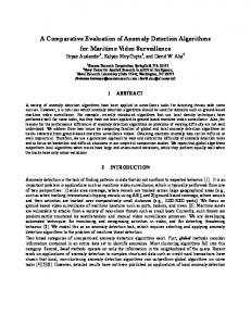
Fig. 1. Shadow detector approaches taxonomy. First the approaches are classified by means of their statistical or non-statistical approach. Further classification for parametric or model-based choose is done. Finally, every approach can be identified by the spectral, spatial and temporal features they exploit.
these four classes. This comparison takes into account both the advantages and the drawbacks of each proposal and provides a quantitative and qualitative evaluation of them. Quantitative (detection and discrimination accuracy) and qualitative metrics (scene and object independence, flexibility to shadow situations and robustness to noise) are proposed to evaluate these classes of algorithms on a benchmark suite of indoor and outdoor video sequences. These video sequences and associated “ground-truth” data are made available at http://cvrr.ucsd.edu:88/aton/shadow to allow for others in the community to experiment with new algorithms and metrics. In the next Section we describe the problem of shadow analysis and discuss a general framework used for shadow detection. In Section 3 we develop a two layer taxonomy for surveying various algorithms presented in literature. Each approach class is detailed and discussed to emphasize its strengths and its limitations. In Section 4, we develop a set of evaluation metrics to compare the shadow detection algorithms. This is followed by Section 5 where we present a results of empirical evaluation of four selected algorithms on a set of five video sequences. The final Section presents concluding remarks. II. S HADOW
PERCEPTION
Shadows are due to the occlusion of the light source by an object in the scene.The part of an object that is not illuminated is called self-shadow, while the area projected on the scene by the object is called
cast shadow and is further classified into umbra and penumbra [7]. The umbra corresponds to the area where the direct light is totally blocked by the object, whereas in the penumbra area it is partially blocked. The umbra is easier to be seen and detected, but is more likely to be misclassified as moving object. If the object is moving, the cast shadow is more properly called moving cast shadow [18]. It has been demonstrated [19]that shadows can be extracted by performing the difference between the current frame sk (at time k) and a reference image s0 , that can be the previous frame, as in [18], or a reference frame, typically named background model [20][21][22]. As reported in [19], under the assumptions of static background and sufficiently strong light source, the difference between a previously illuminated point and the same point covered by a shadow (in the case of umbra) is high. However, the difference result is somewhat similar in the case of foreground points. The approaches in literature differ by means of how they distinguish between foreground and shadow points. Most of these works locally exploit pixel appearance change due to cast shadows [7][21][15][23][18]. A possible approach is to compute the ratio between the appearance of the pixel in the actual frame and the appearance in a reference frame. In [18], authors exploit the assumption of planar background to detect a “possible shadow” searching for uniform region with local constant ratio. The works we will compare start from these assumptions. They can be summarized as the hypothe-
3 Statistical parametric Paper Spectral Friedman and Russell 1997 [26] C Miki´c et al. 2000 [14][24] C
Paper
Spatial L R
Temporal D D
Deterministic model based Spectral Spatial
Temporal
Irvin and McKeown Jr.1 1989 [1] Wang et al. 1991 [5] Kilger 1992 [20] Koller et al. 1993 [16] Onoguchi2 1998 [31]
G G G G G
L R R L L
S S S S S
Statistical non-parametric Paper Spectral Spatial Horprasert et al. 1999 [25] C L Tao et al.4 2000 [27] C R McKenna et al. 2000 [28] C L Deterministic non-model based Paper Spectral Spatial Scanlan et al.1 1990 [29] Jiang and Ward1 1992 [7] Charkari and Mori 1993 [30] Sexton and Zhang 1993 [21] Funka-Lea and Bajcsy1 1995 [32] Sonoda and Ogata 1998 [33] Tzomakas and von Seelen 1998 [34] Amamoto and Fujii 1999 [35] Stauder et al. 1999 [18] Cucchiara et al. 2001 [22]
G G G G G G G G G C
L R R L R R R N/A3 R L
Temporal S D S Temporal S S S S D S S D D S
TABLE I C LASSIFICATION OF THE LITERATURE ON SHADOW DETECTION . M OST OF THE PAPERS PRESENTED IN LITERATURE ARE CLASSIFIED ACCORDING TO THE FOUR CLASSES PROPOSED . T HEIR AUTHORS , THE REFERENCE WORK AND THE YEAR OF PUBLICATION ARE REPORTED AND THE SPECTRAL , SPATIAL AND TEMPORAL FEATURES USED ARE DEPICTED (G= GREY- LEVEL , C= COLOR , L= LOCAL / PIXEL - LEVEL R= REGION - LEVEL , S= STATIC , D= DYNAMIC ).
ses (approximated but realistic) that the light source is white, isotropically scattered within the object and sufficiently strong; moreover, the reference image is assumed static, textured and planar; finally, the objects are considered with perfectly matte surfaces (or Lambertian surfaces). III. TAXONOMY OF SHADOW DETECTION ALGORITHMS
Most of the proposed approaches take into account the described shadow model. To account for their differences, we have organized the various algorithms in a two-layer taxonomy (Fig. 1). The first layer classification considers whether the decision process introduces and exploits uncertainty. Deterministic approaches use an on/off decision process, whereas statistical approaches use probabilistic functions to describe the class membership. Introduc1
This paper considers only still images This paper is not properly a deterministic model approach. It uses an innovative approach based on inverse perspective mapping in which the assumption is that the shadow and the object that casts it are overlapped if projected on the ground plane. Since a model of the scene is necessary, we classify this paper in this class. 3 This paper has the unique characteristic to use the DCT to remove shadow. For this reason, we can say that this paper works on frequencylevel. The rationale used by the authors is that a shadow has, in the frequency domain, a large DC component, whereas the moving object has a large AC component. 4 Since this paper uses a fuzzy neural network to classify points as belonging or not to a shadow, it can be considered a statistical approach. However, how much the parameter setting is automated is not clear in this paper. 2
ing uncertainty to the class membership assignment can reduce noise sensitivity. In the statistical methods (as [14][24][23][25][26]) the parameter selection is a critical issue. Thus, we further divide the statistical approaches in parametric and non-parametric methods. The study reported in [14] is an example of the parametric approach, whereas [23][25] are examples of the non-parametric approach. The deterministic class (see [7][18][22][16]) can be further subdivided. Sub-classification can be based on whether the on/off decision can be supported by model based knowledge or not. Choosing a model based approach achieves undoubtedly the best results, but is, most of the times, too complex and time consuming compared to the non-model based. Moreover, the number and the complexity of the models increase rapidly if the aim is to deal with complex and cluttered environments with different lighting conditions, object classes and perspective views. It is also important to recognize the types of “features” utilized for shadow detection. Basically, these features are extracted from three domains (see Fig. 1): spectral, spatial and temporal. Approaches can exploit differently spectral features, i.e. using gray level or color information. Some approaches improve results by using spatial information working at a region level, instead of pixel level. Finally, some methods exploit temporal redundancy to integrate and improve results.
4
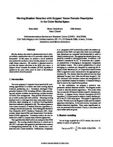
Fig. 2. Flowchart of the S NP algorithm. The first N frames are used to compute, for each pixel, the means and the variances of each color channel, Ei and si respectively. Then, the distortion of the brightness αi and the distortion of the chrominance CDi of the difference between expected color of a pixel and its value in the current image are computed and normalized. Finally, each pixel is classified into four classes using a decision rule based on thresholds automatically computed.
In Table I we have classified 21 papers dealing with shadow detection in four classes. We highlight spectral, spatial and temporal features used by these algorithms. In this paper, we focus our attention on four algorithms (reported in bold in Table I) representative of three of the above-mentioned classes. For the statistical parametric class we choose the algorithm proposed in [14] since this utilizes features from all three domains. The approach reported in [25] can be considered to be a very good representative of the statistical non-parametric class and is also cited and used in [28]. Within the deterministic non-model based class we choose to compare the algorithm described in [22] because is the only one that uses HSV color space for shadow detection. Finally, algorithm reported in [18] has been selected for its unique capability to cope with penumbra. The deterministic model-based class has not been considered due to its complexity and due to its reliance on very specific task domain assumptions. For instance, the approach used in [16] models shadows using a simple illumination model: assuming parallel incoming light, they compute the projection of the 3D object model onto the ground, exploiting two parameters for the illumination direction set offline and assumed to be constant during the entire sequence. However, as stated in [32], in outdoor scene the projection of the shadow is unlikely to be per-
spective, since the light source can not be assumed to be a point light source. Therefore, the need for object models and illumination position’s manual setting make this approach difficult to be implemented in a general-purpose framework. A. Statistical non-parametric (S NP) approach As an example of statistical non-parametric (S NP) approach we chose the one described in [15] and detailed in [25]. This work considers the color constancy ability of human eyes and exploits the Lambertian hypothesis (objects with perfectly matte surfaces) to consider color as a product of irradiance and reflectance. The algorithm is based on pixel modeling and background subtraction and its flowchart is shown in Fig. 2. The first N frames are used to compute, for each pixel, the means and the variances of each color channel. Referring to Fig. 2, Ei = [µR (i), µG (i), µB (i)] is the mean vector and si = [σR (i), σG (i), σB (i)] is the variance vector. The distortion of the brightness αi and the distortion of the chrominance CDi of the difference between expected color of a pixel and its value in the current image Ii = [IR (i), IG (i), IB (i)] are computed as: �
αi =
IR (i)µR (i) 2 (i) σR
�h
i µR (i) 2 σR (i)
+ +
IG (i)µG (i) 2 (i) σG
h
i µG (i) 2 σG (i)
+ +
IB (i)µB (i) 2 (i) σB
h
i µB (i) 2 σB (i)
�
�
(1)
5
Fig. 3. Color model of the D NM 1 approach in the RGB color space. Ei represents the expected color of a given ith pixel and Ii represents the color value of the pixel in the current frame. αi is the brightness distortion and CDi is the chromaticity distortion. According to equation 3, the figure shows the regions detected as foreground (white), background (red), shadows (green) and highlights (blue) in the RGB space.
The rationale used is that shadows have similar chromaticity but lower brightness than the background model. The lower bound in the “foreground” CDi = + rule is introduced to avoid misclassification as shadσR (i) ows of those points of moving objects with very low !2 !2 IG (i) − αi µG (i) IB (i) − αi µB (i) RGB values. Fig. 3 shows the decision rule mapped + + (2) in the RGB color space according to the color model σG (i) σB (i) used. and normalized w.r.t. their root mean square for pixel d . These values are ci and CD i to obtain the values α A statistical learning procedure is used to automati used to classify a pixel in four categories: ically determine the appropriate thresholds. The hisd are built and ci and the CD tograms of both the α i the thresholds are computed by fixing a certain detec d αbi < ταlo , else tion rate. The method proposed is more robust than F oreg. : CDi > τCD or Backg. : α b < τ and αbi > τα2 , else i α1 C(i) = the typical Gaussian distribution-based algorithms; in Shad. : αbi < 0, else d distri ci and the CD fact, the authors show that the α i Highl. : otherwise (3) butions are not Gaussian. v ! u u IR (i) − αi µR (i) 2 t
6
Fig. 4. Flowchart of the S P algorithm. A fading memory estimator calculates background means and variances for all pixel locations. The pdf of a shadowed pixel (ℵ(µSH , σSH )) is estimated from that of a non-shadowed pixel (ℵ(µIL , σIL )) by assuming that v = [R, G, B]T is the value of the pixel not shadowed and by using an approximated linear transformation to estimate the color of the point covered by a shadow. Given the means and the variances for the three color channel for a reference point, the corresponding values under shadows are derived. An iterative probabilistic relaxation to propagate neighborhood information is performed to improve performance. This is achieved by assigning the class membership probabilities in the next iteration using the results of the previous step on the neighborhood pixels.
B. Statistical parametric (S P) approach The algorithm described in [14] for traffic scene shadow detection is an example of statistical parametric (S P) approach and it takes into account most of the assumptions described in Section 2. This algorithm uses two sources of information: local (based on the appearance of the pixel) and spatial (based on the assumption that the objects and the shadows are compact regions). The flowchart of this algorithm is reported in Fig. 4. A fading memory estimator calculates background means and variances for all pixel locations. The pdf of the shadow class is computed by assuming that v = [R, G, B]T is the value of the pixel not shadowed and by using an approximated linear transfor¯ = Dv (where D = diag(dR , dG , dB ) is mation v a diagonal matrix obtained by experimental evaluation) to estimate the color of the point covered by a shadow. The D matrix is assumed approximately constant over flat surfaces. If the background is not
flat over the entire image, different D matrices must be computed for each flat subregion. Given the means and the variances for the three color channels for a reference point, it is straightforward to derive the corresponding values under shadows as µiSH = µiIL di i i and σSH = σIL di , with i ∈ R, G, B. Finally, the aposteriori probabilities of belonging to background, foreground and shadow classes are computed and maximized. This algorithm improves the detection performance by imposing spatial constraints. It performs an iterative probabilistic relaxation to propagate neighborhood information. After this, a post-processing is performed. In this statistical parametric approach the main drawback is the difficult process necessary to select the parameters. Manual segmentation of a certain number of frames is currently done to collect statistics and to compute the values of matrix D. An expectation maximization (EM) approach could be used
7
Fig. 5. Flowchart of the D NM 1 algorithm. The moving object detection is based on background suppression with knowledge-based feedback. The background is computed and updated using a median function over a sequence of previous frames. The knowledge is exploited by updating only those regions previously not detected as moving. Ghosts and ghost shadows are detected and exploited to enhance background updating and shadow detection in the re-shadowing task. The shadow detection is pixel-based and exploit color information in the HSV color space.
to automate this process, as in [26]. C. Deterministic non-model based (D NM 1) approach The system described in [22] is an example of deterministic non-model based approach (we call it D NM 1). The flowchart of the system is reported in Fig. 5. It performs object detection by means of a background suppression and one of its major novelties is the way the background model is computed [12][22]. The model of the background is defined as a combination of statistical and knowledge-based assumptions. A point of the background assumes the value (in the RGB color space) that has the higher probability in a given observation window w = n ·∆t being n the previous frames sampled at a distance of
∆t frames. The more probable value can be detected by using the mode function in a statistically acceptable window. In order to deal with a limited number of samples, the mode function is substituted with the median function that is a good approximation, as has been measured in [12]. The knowledge-based feedback enhances the background update: the points belonging to moving objects detected, validated in their motion state (in order to distinguish them from apparent moving objects) and tracked during time, and the points belonging to moving shadows are not included in the background updating process. The average optical flow computed by the blob analysis (Fig. 5) allows to distinguish between real MVOs (Moving Visual Objects) and apparent MVOs, called ghosts and due to errors in the background modeling. In fact,
8
(a) Ghost shadow scene (raw data)
(b) Ghost shadow scene (highlighted results)
Fig. 6. Ghost shadow example. Ghost shadow scene is reported in (a) and the highlighted results (with an unknown algorithm) in (b), where blue pixels identify shadow points and red pixels belong to a foreground object. Note that this ghost shadow is due to the lower reflection of the cabinet door that has been opened, but was closed in the previous frames. From the intensity point of view this is a shadow since it is due to an intensity decrease.
the background suppression method returns spurious moving objects called ghosts, corresponding to actual background areas incorrectly detected as moving objects. For instance, a stopped car that begins to move will take some frames to be removed from the background: during this period the background suppression will detect as moving object the “ghost” of the car too. The same problem can arise in the case of shadow and is called “ghost shadow” [22]. Fig. 6 reports an example of this special case. In Fig. 6(a) the ghost shadow is due to the lower reflection of the cabinet door that has been opened, but was closed in the previous frames. From the intensity point of view this is a shadow since it is due to an intensity decrease; however, this type of shadow is not due to the occlusion of the light source by an object. Fig. 6(b) reports the result of a shadow detector: the blue area detected as shadow at the bottom of the cabinet door is indeed a ghost shadow. The D NM 1 approach is able to detect shadows and then to classify them as MVO shadows or ghost shadows. In the re-shadowing task (see Fig. 7) only the MVO shadows is excluded from the background update since it does not belong semantically to the background model (see [22] for details). For the shadow detection part (reported in gray in Fig. 5), this algorithm works in the HSV color space. The main reasons are that HSV color space corresponds closely to the human perception of color [36] and it has revealed more accuracy in distinguishing shadows. In fact, a shadow cast on a background does not change significantly its hue [37]. Moreover, the
authors exploit saturation information since has been experimentally evaluated than shadow often lower the saturation of the points. The resulting decision process is reported in the following equation: I V (x,y) 1 if α ≤ BkV (x,y) ≤ β k ∧ (IkS (x, y) − BkS (x, y)) ≤ τS SPk (x, y) = ∧ |IkH (x, y) − BkH (x, y)| ≤ τH 0 otherwise
(4)
where Ik (x, y) and Bk (x, y) are the pixel values at coordinate (x, y) in the input image (frame k) and in the background model (computed at frame k), respectively. The foreground mask Fk (x, y) is set to 1 if the point at coordinates (x,y) is detected as “probably” in motion and, therefore, has to be used both for MVO and for shadow detection. The use of β prevents the identification as shadows of those points where the background was slightly changed by noise, whereas α takes into account the “power” of the shadow, i.e. how strong the light source is w.r.t. the reflectance and irradiance of the objects. Thus, stronger and higher the sun (in the outdoor scenes), the lower α should be chosen. D. Deterministic non-model based (D NM 2) approach Eventually, we compare the approach presented in [18]. This is also a deterministic non-model based approach, but we have included it because its capability of detecting penumbra in moving cast shadow. The flowchart for the shadow detection approach is shown in Fig. 7(a) and is provided by verifying
9
(a) Overview flowchart of the D NM 2 algorithm
(b) Static/moving edge classification flowchart
(c) Uniform shading detection flowchart
(d) Penumbra detection flowchart
Fig. 7. The D NM 2 approach to shadow detection. The gray boxes indicate the three criteria used. The current and previous frame are used to detect static and moving edges, to detect uniform region of shading in the image and to detect penumbra. Then, these criteria are used, together with heuristic rules, to classify every changed region of the image into shadow or no shadow.
three criteria: the presence of static and moving edges (Fig. 7(b)), the presence of “darker” uniform regions (Fig. 7(c)) and the presence of a high difference in luminance w.r.t reference frame. For edge detection, a method inspired by the sensitivity of a human eye to edges is used. A point is detected as edge if it has a zero crossing and a high locally computed variance of the second derivative of the image luminance. Then, a point belonging to an edge is classified as static if the energy in high
frequencies of the frame difference is low in a local neighborhood of the point. Otherwise, the edge point is classified as moving (Fig. 7(b)). Static edges hint at static background and can be exploited to detect nonmoving regions inside the frame difference. According to the assumption that the ratio between frames is locally constant in presence of cast shadows, this algorithm computes the frame ratio for each pixel. If this ratio is locally constant, there is a high probability that the point belongs to a shadow, thus
10
the D NM 2 approach identifies uniform region of the image as possible shadow regions (Fig. 7(c)). Using the classification results from these first two criteria and the change detection mask, each region of the image is classified into 17 different types that consider most of the combination of the changed/unchanged, no edge/static edge/moving edge and no result/uniform/non-uniform hypotheses. By means of some heuristic rules it is decided whether the change is due to moving cast shadows. The rules require changed image regions containing either no edges or static edges and, additionally, a uniform change of shading, at least in a local neighborhood [18]. Finally, to detect penumbra the authors propose to compute the width of each edge in the difference image (Fig. 7(d)). Since penumbra causes a soft luminance step at the contour of a shadow, they claim that the edge width is the more reliable way to distinguish between objects contours and shadows contours (characterized by a width greater than a threshold). This approach is one of the most complete proposed in literature. Nevertheless, in this case the assumptions and the corresponding approximations introduced are strong and they could lack in generality. Also, the penumbra criterion is not explicitly exploited to add penumbra points as shadow points, but it is only used to remove the points that do not fit this criterion. Moreover, the proposed algorithm uses the previous frame (instead of the background) as reference frame. This choice exhibits some limitations in moving region detection since it is influenced by object speed and it is too noise sensitive. Thus, to make the comparison of these four approaches as fair as possible, limited to the shadow detection part of the system, we implement the D NM 2 approach using a background image as reference image, as it was done for the other three approaches. IV. P ERFORMANCE EVALUATION METRICS In this section, the methodology used to compare the four approaches is presented. In order to systematically evaluate various shadow detectors, it is useful to identify the following two important quality measures: good detection (low probability to misclassify a shadow point) and good discrimination (the probability to classify non-shadow points as shadow should be low, i.e. low false alarm
rate). The first one corresponds to minimizing the false negatives (FN), i.e. the shadow points classified as background/foreground, while for good discrimination, the false positives (FP), i.e. the foreground/background points detected as shadows, are minimized. A reliable and objective way to evaluate this type of visual-based detection is still lacking in literature. In [38], the authors proposed two metrics for moving object detection evaluation: the Detection Rate (DR) and the False Alarm Rate (FAR). Assuming T P as the number of true positives (i.e. the shadow points correctly identified), these two metrics are defined as follows: DR =
TP TP + FN
; F AR =
FP (5) TP + FP
These figures are not selective enough for shadow detection evaluation, since they do not take into account whether a point detected as shadow belongs to a foreground object or to the background. If shadow detection is used to improve moving object detection, only the first case is problematic, since false positives belonging to the background do not affect neither the object detection nor the object shape. To account this, we have modified the metrics of equation 5, defining the shadow detection accuracy η and the shadow discrimination accuracy ξ as follows: T PS T PS + F NS T PF ξ= T PF + F NF η=
(6) (7)
where the subscript S stays for shadow and F for foreground. The T PF is the number of ground-truth points of the foreground objects minus the number of points detected as shadows but belonging to foreground objects. In addition to the above quantitative metrics, we also consider the following qualitative measures in our evaluation: robustness to noise, flexibility to shadow strength, width and shape, object independence (it evaluates how many constraints the algorithm imposes on the objects casting the shadows, in particular on their class, speed and dimensions), scene independence, computational load and detection of indirect cast shadows and penumbra. Indirect cast shadows are the shadows cast by a moving object over another moving object and their effect is to
11
Sequence type Sequence length Image size Shadow strength Shadow size Object class Object size Object speed5 Noise level
Highway I
Highway II
Campus
Laboratory
Intelligent room
outdoor 1074
outdoor 1134
outdoor 1179
indoor 987
indoor 900
320x240 medium
320x240 high
352x288 low
320x240 very low
320x240 low
large vehicles large 30-35 medium
small vehicles small 8-15 medium
very large vehicle/people medium 5-10 high
medium people/other medium 10-15 low
large people medium 2-5 medium
TABLE II T HE SEQUENCE BENCHMARK USED . T HE BENCHMARK SHOULD BE COMPLETE AND NOT TRIVIAL TO STRESS THE SHADOW DETECTION CAPABILITIES OF THE APPROACH UNDER COMPARISON . T HE SEQUENCE SET CHOSEN HAS BOTH INDOOR AND OUTDOOR SCENES , INCLUDING LARGE AND SMOOTHED SHADOWS AS WELL AS SMALL AND DARK ONES . I T CONTAINS DIFFERENT OBJECT CLASSES WITH VARIOUS SIZE AND SPEED . T HE LENGTH ( IN NUMBER OF FRAMES ) AND THE SIZE OF THE IMAGES ARE REPORTED . A N EVALUATION OF NOISE IN THE IMAGES OF EACH SEQUENCE IS SHOWN TOO .
decrease the intensity of the moving object covered, order to detect its shadow. probably affecting the object detection, but not the A. Quantitative comparison shadow detection. To compute the evaluation metrics described in V. E MPIRICAL COMPARATIVE EVALUATION Section 4, the ground-truth for each frame is necIn this section, the experimental results and the essary. We obtained it by segmenting the images quantitative and qualitative comparison of the four with an accurate manual classification of points in approaches are presented. As a benchmark, we se- foreground, background and shadow regions. We lect the sequences reported in Table II, where both in- prepared ground truth on tens of frames for each door and outdoor sequences are present, where shad- video sequence representative of different situations ows range from dark and small to light and large and (dark/light objects, multiple objects or single object, where the object type, size and speed vary consider- occlusions or not). Results are reported in Table III. To establish a ably. The Highway I and the Highway II sequences fair comparison, algorithms do not implement any show a traffic environment (at two different lighting conditions) where the shadow suppression is very background updating process (since each tested alimportant to avoid misclassification and erroneous gorithm proposes a different approach). Instead we counting of vehicles on the road. The Campus se- compute the reference image and other parameters quence is a noisy sequence from outdoor campus site from the first N frames (with N varying with the where cars approach to an entrance barrier and stu- sequence considered). Fig. 8 reports the rankdents are walking around. The two indoor sequences ing in shadow detection and shadow discrimination report two laboratory rooms in two different perspec- accuracy derived from Table III. Eventually, the tives and lighting conditions. In the Laboratory se5 The object speed has been measured in average number of pixels per quence, besides walking people, a chair is moved in frame.
12
S NP SP D NM 1 D NM 2
Highway I η% ξ% 81.59% 63.76% 59.59% 84.70% 69.72% 76.93% 75.49% 62.38%
Highway II η% ξ% 51.20% 78.92% 46.93% 91.49% 54.07% 78.93% 60.24% 72.50%
Campus η% ξ% 80.58% 69.37% 72.43% 74.08% 82.87% 86.65% 69.10% 62.96%
Laboratory η% ξ% 84.03% 92.35% 64.85% 95.39% 76.26% 89.87% 60.34% 81.57%
Intelligent Room η% ξ% 72.82% 88.90% 76.27% 90.74% 78.61% 90.29% 62.00% 93.89%
TABLE III E XPERIMENTAL RESULTS . E ACH APPROACH HAS BEEN TESTED ON THE BENCHMARK . F OR EACH EXPERIMENT THE η AND THE SHADOW DISCRIMINATION ACCURACY ξ IN PERCENTAGE ARE REPORTED .
SHADOW DETECTION ACCURACY
(a) Shadow detection accuracy ranking
(b) Shadow discrimination accuracy ranking
Fig. 8. Ranking of the four approaches with regard to the shadow detection accuracy (a) and the shadow discrimination accuracy(b). For each approach the ranking for each sequence is reported.
visual results on a subset of the Intelligent Room and of the Highway I sequences are available at http://cvrr.ucsd.edu:88/aton/shadow. The S NP algorithm is very effective in most of the cases, but with very variable performances. It achieves the best detection performance η and high discrimination accuracy ξ in the indoor sequence Laboratory, with percentages up to 92%. However, the discrimination accuracy is quite low in the Highway I and Campus sequences. This can be explained by the dark (similar to shadows) appearance of objects in the Highway I sequence and by the strong noise component in the Campus sequence. The S P approach achieves good discrimination accuracy in most of the cases. Nevertheless, its detection accuracy is relatively poor in all the cases but the Intelligent room sequence. This is mainly due to the approximation of constant D matrix on the entire image. Since the background can be rarely assumed as flat on the entire image, this approach lacks in generality. Nevertheless, good accuracy in the case of In-
telligent room test shows how this approach can deal with indoor sequences where the assumption of constant D matrix is valid. The D NM 1 algorithm is the one with the most stable performance, even with totally different video sequences. It achieves good accuracy in almost all the sequences. It outperforms the other algorithms in the Campus and in the Intelligent room sequences. The D NM 2 algorithm suffers mainly due to the assumption of planar background. This assumption fails in the case of the Laboratory sequence where the shadows are cast both on the floor and on the cabinet. The low detection performance in the Campus sequence is mainly due to noise and this algorithm has proven low robustness to strong noise. Finally, this algorithm achieves the worst discrimination result in all the cases but the Intelligent room sequence. This is due to its assumption of textured objects: if the object appearance is not textured (or seems not textured due to the distance and the quality of the acquisition system), the probability that parts of the
13
(a) Raw image
(b) S NP result
(c) S P result
(d) D NM 1 result
(e) D NM 2 result
(f) Raw image
(g) S NP result
(h) S P result
(i) D NM 1 result
(j) D NM 2 result
(k) Raw image
(l) S NP result
(m) S P result
(n) D NM 1 result
(o) D NM 2 result
(p) Raw image
(q) S NP result
(r) S P result
(s) D NM 1 result
(t) D NM 2 result
(u) Raw image
(v) S NP result
(w) S P result
(x) D NM 1 result
(y) D NM 2 result
Fig. 9. Results of shadow detection in the indoor sequence Intelligent room. In all these figures, red pixels identify foreground point and blue pixels indicate shadow points.
object are classified as shadow arises. In fact, in the Intelligent room sequence the clothes of the person in the scene are textured and the discrimination accuracy is higher. This approach outperforms the others in the more difficult sequence (Highway II). The statistical approaches perform robustly in noisy data, due to statistical modeling of noise. On
the other hand, deterministic approaches (in particular if pixel-based and almost unconstrained as D NM 1) exhibit a good flexibility to different situations. Difficult sequences, like Highway II, require, however, a more specialized and complete approach to achieve good accuracy. To help evaluating the approaches the results on the Highway I outdoor sequence and on
14
the Intelligent room indoor sequence are available at http://cvrr.ucsd.edu:88/aton/shadow. Fig. 9 shows an example for each sequence. The set of experiments discussed above are useful to evaluate relative performance of the four algorithms, over a wide range of conditions captured by the five test video sequences. It is also important to investigate how shadow detection metrics perform over a large range of frames, within a selected video sequence. Basically, in this case, the nature of shadows, objects, object/shadow movements, illumination effects can all be considered to be relatively constant. Results of such an evaluation are discussed next. Every other of 224 frames of the Intelligent room sequence have been manually segmented. All the 112 manually segmented images are available at http://cvrr.ucsd.edu:88/aton/shadow. The shadow detection accuracy η and the shadow discrimination accuracy ξ over the sequence are shown in Fig. 10 and Fig. 11, respectively. From this extended empirical evaluation is possible to note that while the discrimination accuracy is quite stable, the detection accuracy is more frame-dependent. The main reason is that in this sequence only one object is present, but the shadows are cast on different surfaces and under different conditions. The behaviour of the systems in such different conditions is reported in Fig. 10 where three significant snapshots are shown. First, around frame 100 all approaches but the D NM 2 have an accuracy close to 80%. The reason of the low performance of D NM 2 approach is the detection as object of the shadow close to the person’s feet (Fig. 10): the region spatial connectivity present in this algorithm expands the object classification to the shadow close to the feet, whereas the pixel-based approach (for instance, in the D NM 1 algorithm) avoids this incorrect classification. Around frame 214 there is an interesting anomaly: all the algorithms except the S P suffers degradation in performance, whereas performance of the S P improves. In this frame the shadows are cast under the table and while the statistical parametric approach can detect them (choosing appropriate parameters), the other algorithms can not. The flexibility achievable with a degree of freedom in the parameter selection is shown in the last pair of images (frame 282) where the two statistical approaches are compared. Discrimination accuracy is more stable. Three pairs of snapshots are reported in Fig. 11. The left
one shows why the discrimination accuracy of the D NM 2 approach is higher around frame 134. Some parts of the person are detected as shadow by the other algorithms (as S NP for example), resulting in false positives increase. Moreover, the black hair of the person is misclassified as shadow due to their “dark” appearance. Thanks to its spatial reasoning the D NM 2 approach can deal with this situation. After frame 260, the performance of all the algorithms degrades. The results for the S P and the D NM 1 approaches are reported, showing that the left leg of the person is eroded and partially detected as shadow. In this case the color of the pants is very similar to the chair legs in the background. Object color is usually an important cue to help distinguishing objects from shadows. A similar example is reported in the last pair of images. B. Qualitative comparison To evaluate the behaviour of the four algorithms with respect to the qualitative issues presented in Section 4, we vote them ranging from “very low” to “very high” (see Table IV). The D NM 1 method is the most robust to noise, thanks to its pre- and postprocessing algorithms [22]. The capacity to deal with different shadow size and strength is high in both the S NP and the D NM 1. However, the higher flexibility is achieved by the D NM 2 algorithm which is able to detect even the penumbra in an effective way. Nevertheless, this algorithm is very object-dependent, in the sense that, as already stated, the assumption on textured objects affects strongly the results. Also, the two frame difference approach proposed in [18] is weak as soon as the object speeds increase. The planar background hypothesis makes the D NM 2 and especially the S P approaches more scenedependent than the other two. Although we can not claim to have implemented these algorithms in the most efficient way, the D NM 2 seems the more time consuming, due to the amount of processing necessary. On the other hand, the S NP is very fast. Finally, we evaluated the behaviour of the algorithms in the presence of indirect cast shadows (see Section 4). In Fig. 12 the results in the case of indirect cast shadow are shown. The D NM 2 approach is able to detect both the penumbra and the indirect cast shadow in a very effective way. Note that the penumbra in Fig. 12(e) has been detected as foreground because, accordingly to [18], we use penum-
15
Fig. 10. Shadow detection accuracy of the test on the first 300 frames of the Intelligent room sequence. The first 80 frames are used for the background computation and the collection of the background statistics and thus are not reported in this graph. Every other of the remaining frames have been manually segmented, resulting in 112 samples. Three pairs of image results have been included to help evaluation. The black number in the left-bottom corner of each snapshot represents the frame number, while the green label in the right-bottom corner shows the approach used. Note that the detection performance is far from stable.
Fig. 11. Shadow discrimination accuracy of the test on the first 300 frames of the Intelligent room sequence. The first 80 frames are used for the background computation and the collection of the background statistics and thus are not reported in this graph. Every other of the remaining frames have been manually segmented, resulting in 112 samples. Three pairs of image results have been included to help evaluation. The black number in the left-bottom corner of each snapshot represents the frame number, while the green label in the right-bottom corner shows the approach used. The discrimination performance results more stable than the detection performance. This is mainly due to the presence of a single object in the scene, where the shadow to be detected are cast on several different surfaces and conditions.
16
S NP SP D NM 1 D NM 2
Robustness to noise high high very high low
Flexibility to shadow high medium high very high
Object independence high high high low
Scene independence high low high medium
Computational load very low low low high
Indirect shadow & penumbra detection high low very low very high
TABLE IV Q UALITATIVE EVALUATION . S IX PARAMETERS HAVE BEEN CHOSEN TO OVERVIEW THE FEATURES OF THE APPROACHES PRESENTED . A VOTE FROM “ VERY LOW ” TO “ VERY HIGH ” TO EACH APPROACH HAS BEEN GIVEN FOR EACH PARAMETER .
(a) Raw image
(b) S NP result
(c) S P result
(d) D NM 1 result
(e) D NM 2 result
Fig. 12. Results on indirect cast shadow. In the case of moving shadow casts on a moving object, the four algorithms behave in a different way. The S P algorihtm detects correctly most of the indirect cast shadow (Fig. (b)), where the S NP (Fig. (c)) and the D NM 1 (Fig. (d)) algorithms do not. The best detection is achieved by the D NM 2 method (Fig. (e)). In all these figures, red pixels identify foreground point and blue pixels indicate shadow points.
bra information only to assert the classification process and not to detect penumbra points. The S P and the D NM 1 methods failed in detecting indirect cast shadows. The pixel-based decision can not distinguish correctly between this type of moving shadows and those shadows cast on the background. However, the S P approach is able to detect relatively narrow penumbra. VI. C ONCLUDING REMARKS Development of practical dynamic scene analysis systems for real-world applications needs careful consideration of the moving shadows. Research community has recognized this and serious, substantive efforts in this area are being reported. The main motivator for this paper is to provide a general framework to discuss such contributions in the field and also to provide a systematic empirical evaluation of a selected representative class of shadow detection algorithms. In this paper an overview of moving shadow detection problem is presented. Papers dealing with shadows are classified in a two-layer taxonomy and four representative algorithms are described in detail. A set of novel quantitative and qualitative metrics has been adopted to evaluate the approaches. We performed an extensive empirical study using five video sequences, to evaluate efficacy of the new metrics in
judging four selected shadow detection algorithms. Main conclusion of the empirical study can be described as follows. For a general-purpose shadow detection system, with minimal assumptions, a pixel based deterministic non-model based approach (D NM 1) assures best results. On the other hand, to detect shadows efficiently in one specific environment, more assumptions yield better results and deterministic model-based approach should be applied. In this situation, if the object classes are numerous to allow modeling of every class, a complete deterministic approach, like the D NM 2, should be selected. If the environment is indoor, the statistical approaches are the more reliable, since the scene is constant and a statistical description is very effective. If there are different planes onto which the shadows can be cast, an approach like S NP is the best choice. If the shadows are scattered, narrow, or particularly “blended” to the environment, a region-based dynamic approach, typically deterministic, is the best choice (as D NM 2 in the Highway II scene reported in this paper). Finally, if the scene is noisy, a statistical approach or a deterministic approach with effective pre- and post-processing steps should be used. Finally, we want to remark that all the evaluated approaches exploit a large set of assumptions, to limit complexity and to avoid being undully constrained
17
to a specific scene model. This limits their shadow detection accuracies. This in fact points to the limitations of using only image-derived information in shadow detection. Further improvements would require feedback of specific task/scene domain knowledge. ACKNOWLEDGMENTS Our research is supported in part by the California Digital Media Innovation Program (DiMI) in partnership with the California Department of Transportation (Caltrans), Sony Electronics, and Compaq Computers. We wish to thank our collaborators from the Caltrans (TCFI) in Santa Barbara for their support and interactions. We extend special thanks to our colleagues in the CVRR Laboratory for their efforts in acquiring the video data sets utilized in our studies. R EFERENCES [1]
[2] [3] [4] [5] [6] [7] [8]
[9] [10]
[11] [12]
[13]
R.B. Irvin and D.M. McKeown Jr., “Methods for exploiting the relationship between buildings and their shadows in aerial imagery,” IEEE Transactions on Systems, Man, and Cybernetics, vol. 19, pp. 1564–1575, 1989. A. Huertas and R. Nevatia, “Detecting buildings in aerial images,” Computer Vision, Graphics and Image Processing, vol. 41, pp. 131–152, Feb. 1988. Y. Liow and T. Pavlidis, “Use of shadows for extracting buildings in aerial images,” Computer Vision, Graphics and Image Processing, vol. 49, no. 2, pp. 242–277, Feb. 1990. G. Medioni, “Obtaining 3-D from shadows in aerial images,” in Proceedings of IEEE Int’l Conference on Computer Vision and Pattern Recognition, 1983, pp. 73–76. C. Wang, L. Huang, and A. Rosenfeld, “Detecting clouds and cloud shadows on aerial photographs,” Pattern Recognition Letters, vol. 12, no. 1, pp. 55–64, Jan. 1991. S.A. Shafer and T. Kanade, “Using shadows in finding surface orientations,” Computer Vision, Graphics and Image Processing, vol. 22, no. 1, pp. 145–176, Apr. 1983. C. Jiang and M.O. Ward, “Shadow identification,” Proceedings of IEEE Int’l Conference on Computer Vision and Pattern Recognition, pp. 606–612, 1992. Y. Kameda and M. Minoh, “A human motion estimation method using 3-successive video frames,” in Proceedings of International Conference on Virtual Systems and Multimedia, 1996, pp. 135– 140. R.C. Jain, “Difference and accumulative difference pictures in dynamic scene analysis,” Image and Vision Computing, vol. 2, no. 2, pp. 99–108, May 1984. R. Cucchiara, M. Piccardi, and P. Mello, “Image analysis and rule-based reasoning for a traffic monitoring system,” IEEE Transactions on Intelligent Transportation Systems, vol. 1, no. 2, pp. 119–130, June 2000. A. Neri, S. Colonnese, G. Russo, and P. Talone, “Automatic moving object and background separation,” Signal Processing, vol. 66, no. 2, pp. 219–232, 1998. R. Cucchiara, C. Grana, M. Piccardi, and A. Prati, “Statistical and knowledge-based moving object detection in traffic scene,” in Proceedings of IEEE Int’l Conference on Intelligent Transportation Systems, Oct. 2000, pp. 27–32. A. Bainbridge-Smith and R.G. Lane, “Determining optical flow
[14] [15]
[16]
[17] [18] [19]
[20] [21] [22]
[23] [24]
[25]
[26] [27]
[28] [29]
[30] [31] [32] [33]
using a differential method,” Image and Vision Computing, vol. 17, pp. 11–22, 1997. I. Mikic, P. Cosman, G. Kogut, and M.M. Trivedi, “Moving shadow and object detection in traffic scenes,” in Proceedings of Int’l Conference on Pattern Recognition, Sept. 2000. I. Haritaoglu, D. Harwood, and L.S. Davis, “W4: real-time surveillance of people and their activities,” IEEE Transactions on Pattern Analysis and Machine Intelligence, vol. 22, no. 8, pp. 809–830, Aug. 2000. D. Koller, K. Daniilidis, and H.H. Nagel, “Model-based object tracking in monocular image sequences of road traffic scenes,” International Journal of Computer Vision, vol. 10, pp. 257–281, 1993. C. Tomasi and T. Kanade, “Detection and tracking of point features,” Tech. Rep. CMU-CS-91-132, Carnegie Mellon University, 1991. J. Stauder, R. Mech, and J. Ostermann, “Detection of moving cast shadows for object segmentation,” IEEE Transactions on Multimedia, vol. 1, no. 1, pp. 65–76, Mar. 1999. A. Prati, I. Mikic, C. Grana, and M.M. Trivedi, “Shadow Detection Algorithms for Traffic Flow Analysis: a Comparative Study,” in Proceedings of IEEE Int’l Conference on Intelligent Transportation Systems, Aug. 2001, pp. 340–345. M. Kilger, “A shadow handler in a video-based real-time traffic monitoring system,” Proceedings of IEEE Workshop on Applications of Computer Vision, pp. 11–18, 1992. G.G. Sexton and X. Zhang, “Suppression of shadows for improved object discrimination,” in Proc. IEE Colloq. Image Processing for Transport Applications, Dec. 1993, pp. 9/1–9/6. R. Cucchiara, C. Grana, M. Piccardi, and A. Prati, “Detecting objects, sahdows and ghosts in video streams by exploiting color and motion information,” in Proceedings of the IEEE Int’l Conference on Image Analysis and Processing, to appear, 2001. A. Elgammal, D. Harwood, and L.S. Davis, “Non-parametric model for background subtraction,” in Proceedings of IEEE ICCV’99 FRAME-RATE Workshop, 1999. M.M. Trivedi, I. Mikic, and G. Kogut, “Distributed video networks for incident detection and management,” in Proceedings of IEEE Int’l Conference on Intelligent Transportation Systems, Oct. 2000, pp. 155–160. T. Horprasert, D. Harwood, and L.S. Davis, “A statistical approach for real-time robust background subtraction and shadow detection,” in Proceedings of IEEE ICCV’99 FRAME-RATE Workshop, 1999. N. Friedman and S. Russell, “Image segmentation in video sequences: a probabilistic approach,” in Proceedings of the 13th Conference on Uncertainty in Artificial Intelligence, 1997. X. Tao, M. Guo, and B. Zhang, “A neural network approach to the elimination of road shadow for outdoor mobile robot,” in Proceedings of IEEE Int’l Conference on Intelligent Processing Systems, 1997, vol. 2, pp. 1302–1306. S.J. McKenna, S. Jabri, Z. Duric, A. Rosenfeld, and H. Wechsler, “Tracking groups of people,” Computer Vision and Image Understanding, vol. 80, no. 1, pp. 42–56, Oct. 2000. J.M. Scanlan, D.M. Chabries, and R.W. Christiansen, “A shadow detection and removal algorithm for 2-D images,” in Proceedings of Int’l Conference on Acoustics, Speech and Signal Processing, 1990, vol. 4, pp. 2057–2060. N.M. Charkari and H. Mori, “A new approach for real time moving vehicle detection,” in Proceeding of IEEE/RSJ Int’l Conference on Intelligent Robots and Systems, 1993, pp. 273–278. K. Onoguchi, “Shadow elimination method for moving object detection,” in Proceedings of Int’l Conference on Pattern Recognition, 1998, vol. 1, pp. 583–587. G. Funka-Lea and R. Bajcsy, “Combining color and geometry for the active, visual recognition of shadows,” in Proceedings of IEEE Int’l Conference on Computer Vision, 1995, pp. 203–209. Y. Sonoda and T. Ogata, “Separation of moving objects and their shadows, and application to tracking of loci in the monitoring im-
18
[34]
[35]
[36]
[37]
[38]
ages,” in Proceedings of Int’l Conference on Signal Processing, 1998, pp. 1261–1264. C. Tzomakas and W. von Seelen, “Vehicle detection in traffic scenes using shadows,” Tech. Rep. 98-06, IR-INI, Institut fur Nueroinformatik, Ruhr-Universitat Bochum, FRG, Germany, Aug. 1998. N. Amamoto and A. Fujii, “Detecting obstructions and tracking moving objects by image processing technique,” Electronics and Communications in Japan, Part 3, vol. 82, no. 11, pp. 28–37, 1999. N. Herodotou, K.N. Plataniotis, and A.N. Venetsanopoulos, “A color segmentation scheme for object-based video coding,” in Proceedings of the IEEE Symposium on Advances in Digital Filtering and Signal Processing, 1998, pp. 25–29. R. Cucchiara, C. Grana, M. Piccardi, A. Prati, and S. Sirotti, “Improving shadow suppression in moving object detection with HSV color information,” in Proceedings of IEEE Int’l Conference on Intelligent Transportation Systems, Aug. 2001, pp. 334–339. G. Medioni, “Detecting and tracking moving objects for video surveillance,” in Proceedings of IEEE Int’l Conference on Computer Vision and Pattern Recognition, 1999, vol. 2, pp. 319–325.