shadows being cast by objects in motion on a planar sur- face that utilizes the .... blowing in the wind) and the systems ability to suppress non-foreground pixels ...
Moving Shadow Detection using a Combined Geometric and Color Classification Approach ∗ Kideog Jeong and Christopher Jaynes Department of Computer Science and Center for Visualization and Virtual Environments University of Kentucky, Lexington KY Email: {kideog.jeong, jaynes}@vis.uky.edu
Abstract Automatic detection of moving objects is a fundamental problem in computer vision. Motion analysis, object recognition, and video surveillance applications often depend on reliable segmentation of moving objects against a fixed background. Although shadows move in the scene with the objects that cast them, it is often important that only objects in motion, and not their shadows, are detected. For example, false positives of moving shadows that are generated by current approaches to motion segmentation can lead to erroneous object models that will ultimately impact recognition rates. We present an algorithm for the automatic detection of shadows being cast by objects in motion on a planar surface that utilizes the additional geometric information afforded by two views of the scene. Foreground pixels are first generated by an existing motion segmentation method in each of the two views. Moving pixels that have no parallax lie in the ground plane and are considered to be potential shadow pixels. A subset of these shadow pixels is used as input to construct an adaptive mixture color probability model. Once the shadow color model is acquired, it can then be used to efficiently detect shadows in successive frames in conjunction with the zero parallax constraint. The approach has been tested in several different video surveillance scenarios. Results demonstrate that approximately 94 percent of shadow pixels can be correctly classified with small false positive rates.
(a)
(b)
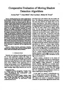
Figure 1: Shadows are a significant problem for motion segmentation and video surveillance applications. As objects move against a static background, their shadows are often detected as foreground pixels. (a) Object shadows can take on similar intensity and color as other objects in the scene (i.e. dark markings on the coffee mug). (b) Even under diffuse lighting, shadows can confound traditional segmentation algorithms.
and object tracking. Oftentimes, an appearance model of the object in motion is constructed directly from the segmented pixel values. As segmentation accuracy degrades, the model will include pixels that are not part of the object and the result is a degradation in the model. This is particularly a problem in the challenging environments encountered in many video surveillance applications. Unknown illumination, including both diffuse and point sources, induce moving shadows that appear “attached” to the objects that cast them. As a result, traditional motion segmentation algorithms often classify shadowed background pixels as foreground. Certainly, shadows move in the scene in conjunction with object or light source motion. This poses a significant challenge to motion detection algorithms that are primarily concerned with tracking or detecting motion based on locally changing intensity patterns alone. Figure 1 depicts the problem we are addressing. Although it may seem that dark shadows may be detected via
1 Introduction In many computer vision applications, moving object detection is either an important goal in itself or is a critical component for other vision tasks. Examples include motionbased object recognition, structure and motion estimation, ∗ This work was funded by NSF CAREER Award IIS-0092874 and by The Kenucky Office of the New Economy
1
simple analysis of pixel luminance (see Figure 1(a)), distinguishing these shadows from pixels with similar color and intensity on an object is difficult. Even environments with fairly diffuse lighting, shown in Figure 1(b), can cause problems as the presence of an object casts shadows on the ground. In order to address this, we introduce a technique that automatically detects pixels corresponding to moving shadows in the scene. We assume that cast shadows fall on a planar surface and that two stationary cameras observe the scene. The utilization of more than one view is not overly restrictive and follows the trend of modern video surveillance systems that are beginning to exploit the availability of low-cost cameras. Dense and wide-area camera networks are emerging to provide ubiquitous coverage of areas under surveillance [1]. This method is intended for domains such as these. Background modeling is an active area of research and is not the focus of the work here. In fact, any system capable of reliable detection of pixels in motion can be used for the foreground detection phase. For example, we demonstrate in Section 4 how the result of density filter estimation is an appropriate input to the shadow detection system [2]. In this paper, we introduce a new foreground detection method that was designed specifically for both speed and a low number of false positives to support our efforts in detecting pixels in shadow at real-time rates. Given a set of foreground pixels detected in two views of the same scene, the approach determines which pixels lie on the world ground plane and are likely to be shadows as opposed to other scene motion pixels that will exhibit parallax above the ground plane in the two views. This additional geometric constraint will both help bootstrap a color model of pixels in shadow as well as provide additional information that will help to segment shadows from objects that have similar appearance. During an initial training phase, pixels that satisfy the planar constraint are used to build an adaptive statistical color model of pixels in shadow. This training phase only requires a few frames and is fully automatic. Subsequent frames then undergo a two-phased tracking process. First, foreground pixels are produced by a foreground detection algorithm. These foreground pixels are then classified as shadow/non-shadow using a statistical test that takes into account how well the pixel conforms to both the planar constraint and the acquired color model. The best matching pixels are used to update the shadow color model. The method is demonstrated against a number of different tracking scenarios including typical indoor ambient lighting and strong point light sources. Although a primary goal of the work is to yield better overall foreground segmentation, explicit labeling of shadow pixels can have utility in itself. We speculate that reliable labeling of pixels in shadow may provide valuable information about light
source intensity and position estimation as well as a source of information about the expected appearance of pixels in shadow for a given scene. These color models may be used for synthetic shadow generation for video editing.
1.1
Related work
Given the problems that shadows can cause for tracking and recognition of objects in motion, several approaches to moving shadow detection have been proposed. Primarily, these techniques utilize a single camera, and model either the chromatic effects or expected intensity variation of pixels in shadow. Systems range from fairly straightforward methods of analyzing intensity via series of different thresholds [3] to more complex pixel classifiers that need a significant set of training data, either collected via some automatic procedure [4] or via a manual setup phase [5]. It should be pointed out that our method is quite different in that we utilize a second camera, and the geometric constraints that can then be enforced on many of the shadows found in a scene. A good example of a chromatic classification approach uses intensity in conjunction with normalized blue and red components to classify pixels as as background, foreground, or shadow [4]. This approach utilizes a probability distribution model to maximize the posterior probability that a particular pixel belongs to one of the three classes. Although the method works quite well in removing spurious background pixels, the reliance on a single color model can lead to mis-classification of shadow pixels, particularly in the presence of specular highlights. In similar work, Horprasert et. al. [3], proposes a color model that compares intensity to the chromaticity component at each pixel. Each pixel is classified as background, shaded, highlighted, and moving foreground through the combination of three threshold values which are defined from a single Gaussian distribution. This method is useful for fast classification of potential shadow regions and has been shown to work quite well under normal lighting conditions. Because intensity plays an important role in determining what pixels are to be classified as shadow, however, the method begins to fail in regions with low total intensity and chromaticity values can change dramatically. A more recent approach emphasizes the importance of carrying out operations in HSV space in order to be robust to lower intensity regions [5]. The work is similar to [3], but utilizes a more sophisticated thresholding scheme to detect shadow pixels. A pixel is classified as shadow if its luminance channel, normalized by the luminance of the background, falls between two predetermined thresholds. In addition the difference between the saturation and hue of a foreground pixel and its corresponding background values must both be less than two thresholds. The method yields a false positive rate of approximately 27 percent. This may be 2
due to the use of a set of thresholds, acting as linear decision boundaries, when the luminance and saturation response in the image can be highly nonlinear in dark or over saturated pixels. Elgammal et al. [6], explicitly takes into account pixels in shadow as part of a more comprehensive foreground detection system based on density kernel estimation. The normalized red and green values are used to lessen the effect of saturation differences caused by potential shadow. In addition, the sum of the RGB values are taken into account to compensate for color measurements of pixels that may be near saturation. The foreground segmentation approach overall has been shown to perform well in challenging conditions including partly changing backgrounds (i.e. leaves blowing in the wind) and the systems ability to suppress non-foreground pixels is impressive. The shadow detection component of the approach, however, generates a significant number of false positives in regions where green and red values are small, leaving the blue channel to be the dominant color. This occurs in dark regions near objects that are in deep shadow and leads to inevitable misclassification of shadow pixels as foreground.
Once the planar projection between the two cameras is known, training is initiated in which objects and their shadows are detected in each view independently. Using the known homography, foreground pixels in each view are warped to a corresponding location in a second view and measured for color consistency via a similarity score. If the pixels are dissimilar, we assume this is due to parallax above the ground-plane and these pixels are marked as foreground. Pixels are sorted by their consistency and the best are used to develop a shadow color model that characterizes the expected color distribution of pixels in shadow. During run-time, foreground pixels are extracted followed by a noise filtering phase. The remaining pixels are warped through the homography to compute a similarity score. This similarity score as well as the color model for shadows are taken into account during shadow classification.
2.2
Using the ground-plane that is observed in each camera, the homography Hab that relates image points in camera a directly to points in image b is recovered via a set of matchpoints known to lie on the world ground-plane. Given points on the same world plane, seen in the two cameras, the relationship between image coordinates in each view can be described as:
2 Technical details A fundamental difference between the method introduced here and previous work is the use of multiple views of the scene to constrain the search for potential shadow pixels. If we assume shadows fall on a planar surface, a planar projection governs how pixels in one view will map to positions in the second view. Of course pixels that do not correspond to world points on this plane will map to points in a second view that no longer correspond. Analysis of this parallax yields what foreground regions may be shadow and what regions are truly “objects” off of the ground. This observation increases the robustness of our system over methods that rely exclusively on color and intensity models. Although geometric analysis is important by itself, it is insufficient and must be combined with a color model that is acquired during a training phase and then updated as cast shadows fall on different colored surfaces in the scene. These two metrics can then be combined into a single classifier that determines what pixels are in shadow for a given scene.
2.1
Ground-plane camera calibration
pˆba = Hab pa
(1)
where H is a 3×3 homography matrix of a projective transformation for the coplanar surface, pa = [u, v, 1]T is a point in camera a and pˆba = [w0 u0 , w0 v 0 , w0 ]T is the corresponding point in camera b, and w 0 is the scale factor used to find the normalized image position of point pˆba , seen in image b; [u0 , v 0 ]. For points that do not lie on this ground-plane, the mapping in Equation (1) does not hold. Figure 2 depicts the behavior of points that are mapped through a homography corresponding to a world ground-plane. By multiplying points in the left image by the homography to discover their corresponding location in the second view, we can see how points on the plane correctly correspond (shown in red), while world points not on the ground-plane, shown in green, (i.e. the set of points selected on the subject’s leg or along the door frame) lead to additional parallax and image points no longer correspond correctly. This geometric transfer function will provide the system with the ability to determine what pixels in motion may lie on the world ground. Other mappings can be used when the local ground-plane assumption is inappropriate and we are extending the approach to take these into account for the future work. For example, a family of homographies
Algorithmic Approach
Cameras must have significant overlap between their view frustums and observe the ground-plane in addition to subjects in motion. This is often the case encountered in traditional multi-view surveillance scenarios (for example Figure 2). The method requires that a planar homography of the ground plane between the two views is initially known. 3
(a)
(b)
Figure 2: A typical two-camera surveillance setup. Pixels mapped from the left view via a homography that corresponds to the world ground-plane will yield a set of correspondences in the right view. If the point is indeed on the world ground-plane (shown in red), pixels in each view will correspond to the same world location. Other pixels (shown in green) will map to incorrect locations in the second view.
can describe the expected mappings for the piecewise planar scenes often encountered in indoor settings (see Section 5). Although we have previously introduced a multi-view calibration technique that can derive the homography automatically in video surveillance scenarios [7], here we use a simple interactive method for experimental purposes. In order to compute a planar homography H, at least four non-aligned correspondence points are required since H has eight degrees of freedom. The user is presented with views from each camera and uses a simple GUI to select corresponding points on the ground-plane in each camera. Once four points have been selected, a homography can be estimated. Then the user is presented with the position of corresponding pixels via the estimated homography. By visualizing the accuracy of the homography via the image re-projection error, a user can iteratively improve the current homography estimate by adjusting the position of match-points in error or by adding new match-points. Once satisfied, the current homography is stored for use during run-time.
2.3
yields and appropriate set of pixels for input to the system.
2.4
Run time detection of foreground pixels
A background model is initially constructed in each view independently. We build a statistical background model similar to that described in [2] at each pixel in RGB space by measuring pixel color values over a short span of time. A set of foreground pixels is generated by evaluating each pixel’s color distribution against its corresponding background model. If a given pixel differs from two standard deviations of the mean of the background model, then it is classified as foreground. Otherwise, we assume that it belongs to background and is no longer considered. The technique has been shown to be capable of generating foreground pixels at real-time rates [2] but is sensitive to small radiometric differences due to noise that cannot be detected using this heuristic. This results in a tradeoff between classification accuracy and computational cost. To overcome the difficulty, we propose an efficient method to reduce noise pixels in the foreground set. A similarity score, between each potential foreground pixel and its correspondence in a mean background model, is measured. The mean background model, Bm , is the mean value of the highest weighted Gaussian distribution at every coordinate in the image. Given the mean background model, Bm , and a set of foreground candidates in F , the normalized sum of squared ˜ , is computed between the foreground candidifferences, N date of the current frame and the mean background over a neighborhood window of size w × w, centered at (u, v).
Background modeling
Background modeling and segmentation of foreground pixels is an active area of research and a number of techniques have been developed [8, 9, 10, 2]. These methods have met varying success and have been developed for a variety of conditions including fast foreground segmentation for object tracking and highly dynamic scenes that require more sophisticated models [2]. Because our method takes an initial set of foreground pixels and then attempts to remove those in shadows, any of these foreground detection methods [8, 9, 10, 2] can be used as input. However, it is important that these systems do not overly eliminate object pixels in an attempt to remove spurious or shadow pixels because our system is capable of doing this in a post processing step without removing pixels on the object. In this paper, we develop an extension of the foreground segmentation method [2] that is efficient and
˜ (F (u, v), Bm (u, v)) = N Pu+s,v+s
x=u−s,y=v−s (F (x, y)
qP
(2) 2
− Bm (x, y)) P u+s,v+s 2 u+s,v+s 2 x=u−s,y=v−s F (x, y) x=u−s,y=v−s Bm (x, y)
where w is an odd integer and s = (w − 1)/2. ˜ less than some fixed threshold, Tnoise , For values of N the corresponding foreground pixel at (u, v) is eliminated 4
ized sum of the squared differences of small pixel neighborhoods centered around the corresponding image points. This linear transform between views, H, and subsequent Sab (pa ) score is computed for all foreground pixels in image a as well as a corresponding similarity score, Sba (pb ), for all foreground pixels in image b compared to image a. The ¯ for both measures is compared to a mean similarity score M predefined threshold, Tshadow . Pixels exceeding this threshold are classified as object in both views and are not considered as shadows. Since the threshold Tshadow decides whether the pixel is to be foreground or moving shadow, it should be chosen with care. For that reason, we determine an optimal threshold by conducting a performance analysis. The details of this process is discussed in Section 3.
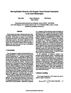
from the foreground set. For the results shown here, the window size, w, is three pixels and seems to provide the similarity score with enough information to remove a significant number of noise pixels from the foreground. The threshold value Tnoise should be small to retain as many pixels of true foreground objects but must discriminate noise pixels from foreground blob pixels. For this work, we conducted a performance analysis to determine an optimal noise threshold as described in Section 3. Figure 3 shows the results of our frame-rate foreground detection system. Figure 3(a) shows pixels (white) that differ from two standard deviations of the mean of the Gaussian color model. Noise suppression then removes a significant number of these pixels without undue processing requirements. The resulting foreground pixels, Fnoise−suppressed , are shown in Figure 3(b).
(a)
2.6
Ideally, all shadow pixels would be detected during the foreground analysis or by removing pixels that do not conform to the planar perspective induced by the ground-plane in each view. However, geometric constraints must be combined with an appearance model of the shadow pixels. Because moving shadows only occur at run-time (as objects move into the scene), a color model of shadow pixels must be built iteratively and then maintained as shadows are detected. To address the problem, we propose a separate intermediate stage for extracting a shadow model (a mixture of Gaussians). The model is extracted through the following two steps: Ks Gaussian distributions are estimated given moving shadow samples, and then meaningful Gaussian distributions are selected to be the shadow model. These initial moving shadow samples are computed automatically using only the geometric consistency measure as described in Section 2.5. This set of pixels, Xinit , where each member is an RGB color pixel, are used as input for estimating the initial color model. We initialize the parameters of Ks Gaussian distributions Θ with a random guess and run maximum-likelihood estimation (MLE) using the Expectation-Maximization (EM) algorithm [11]. This estimation iterates until the likelihood is no longer significantly improved. This results in a set of Ks Gaussian parameters Θ = {ω1 , .., ωKs , µ1 , .., µKs , Σ1 , .., ΣKs }, where ωl is the prior probability (weight), µl is the Σl is the covariance PKmean, s ωl = 1. matrix of lth Gaussian, and l=1 The value of Ks should be chosen to accommodate the number of meaningful Gaussian distributions expected to be covered by the pixels in the shadow collection phase. This is related to the expected color variability both due to material properties of the ground-plane and lighting changes as the object moves through the scene. For the results shown here, we set Ks to 7.
(b)
Figure 3: Result of the noise reduction phase of processing. (a) Foreground detection prior to noise reduction. (b) Remaining foreground pixels after noise reduction has been applied. Dense regions of moving cast shadows still remain in the foreground set.
2.5
Shadow color model acquisition
Initial shadow detection
Moving shadow detection, using only the geometric constraint, runs for the first several of frames as objects enter the scene, in order bootstrap an initial shadow color model. Foreground pixels, Fnoise−suppressed , during this phase are classified into two categories, moving shadow and moving object, in each frame. The parallax off of the ground-plane is measured for each foreground pixel by evaluating pixel’s similarity across two views through the planar homography recovered using the method described in Section 2.2. The geometric constraint not only assists in selecting appropriate pixels for an initial shadow color model, but is used at run-time to continuously filter foreground pixels based on the planar perspective assumption (see Section 2.7). Given the image coordinates of a point in image a, pa , its corresponding pixel location in image b, pˆba is computed via Hab . If pa is located on the world ground-plane, both image pixels should correspond to the same world point. Assuming a Lambertian ground, and cameras with similar spectral response, there should only be a small difference in the color values at pa and pˆba . The similarity score at pa when mapped from image a to b, written as, Sab (pa ) is the normal5
Once the set of parameters Θ have been estimated for the Ks Gaussian distributions, we determine the most meaningful Gaussian distributions to be used in the shadow color model using a technique similar to that described in [2]. The Ks distributions are sorted in descending order of ωs /σs 2 where σs 2 is the variance of mode s. The top ks Gaussian distributions are added to the shadow model, Sshadow−model , until the sum of their weights exceeds a constant value Cshadow . By doing this, we can acquire the most meaningful Gaussian distributions. A good choice for Cshadow can be estimated as the accuracy measured in our performance analysis in Section 3.
2.7
markings on the ground plane may yield new colors not previously seen in the shadow model as a subject moves through the field of view. Ideally, the batch EM algorithm described in Section 2.6 should yield accurate estimate of the shadow colors but it is considered too computationally expensive for run-time updating to be feasible. To overcome the drawback, we propose an adaptive leader-follower clustering [12] technique to update the Gaussian parameters of our shadow model. A set of new candidate shadow pixels is found in each frame during run-time of the shadow classification in Section 2.7. Only pixels that satisfy the first condition but not the second condition in Equation (3) are added to the set. These pixels are likely to be shadows moving on the ground-plane but are not incorporated into the shadow color model. Using the top k-percent of these pixels, Xnew , in ˜ , the color each frame, sorted by their similarity scores, N model is updated. In order to find the best distribution s in the shadow model for each new pixel, x ∈ Xnew , we measure a likelihood score as follows: ¶ µ ωl log 1 d (4) s = arg max (2π) 2 |Σl | 2 l > −1 1 − 2 (x − µl ) Σl (x − µl )
Run time detection of moving shadows
Although geometric analysis by itself is capable of detecting a large number of pixels moving on the ground-plane, the shadow color model is capable of reducing false positives that are likely to occur when pixels that correspond have accidental color similarity. All pixels that are classified as potential foreground via the foreground detection algorithm. These are then compared to the current shadow color model. A potential shadow pixel must meet the following conditions to be classified as shadow.
where d is the dimension of x. After the evaluation for each pixel, only the parameters of distribution s are updated by the following update rule similar to that of [2]:
Fshadow (pa ) = ˜ (I(pa ), I(ˆ pba )) < Tshadow and 1 If N T (C(pa ) − µl ) Σl −1 (C(pa ) − µl ) ≤ δ 2 (3) 0 otherwise
˜ is the normalized where Fshadow is the shadow mask, N sum of squared differences described in Equation (2), I(pa ) and I(ˆ pba ) are the image patches centered at pa and pˆba respectively, C(pa ) is the color value at point pa , µl and Σl is the mean and the the covariance matrix of the l th shadow distribution in Sshadow−model respectively, and δ is the distance threshold. ˜ in the criterion is to The purpose of the first condition N prevent pixels belonging to other planes or moving objects from being misclassified as moving shadows. The next condition is to evaluate the similarity between pixel at pa with respect to each shadow distribution in the shadow model Sshadow−model . The threshold δ can be adjusted depending on the accuracy of the camera and the environments of the application. For our experiments, we set δ to 4. Finally, we label out moving shadow pixels by masking with Fshadow on Fnoise−suppressed from Section 2.4 to have a shadow-free foreground object scene.
2.8
ωˆs = (1 − λ)ωs + λ
(5)
µˆs = (1 − κ)µs + κx ˆ Σs = (1 − κ)Σs + κ((x − µˆs )T Σ−1 s (x − µˆs ))
(6) (7)
where the adaptation factor is defined as κ = λ/ωˆs , λ is a adaptation rate, ω, µ and Σ are the weight, the mean, and the covariance of the Gaussian distribution s respectively. The weights of the shadow model are normalized after update.
3 Determining system parameters In this section, we include some details of Receiver Operating Characteristic (ROC) analysis to demonstrate how appropriate threshold parameters were selected for the system. System parameters include the threshold to determine if a foreground pixel should be filtered as noise, Tnoise , the threshold to determine if corresponding pixels (via the homography) are similar enough to classified as shadow, Tshadow , and other parameter Cshadow that determines how many modes will be used in the Gaussian color models. Cshadow can be simply estimated from the true positive (TP) rate given by a selection of Tshadow . The two thresholds can have a significant impact on the performance of
Shadow color model update
As lighting conditions in the observed scene change, the color of moving shadow regions also changes. Surface 6
the system and need to be selected through an experiment as follows. Ground truth data was initially collected by segmenting foreground objects with respect to our background model for thirty frames. A user then hand edited the foreground regions to remove spurious pixels and then label moving shadow regions as well as foreground objects. This set of ground truth frames can then be used to perform ROC analysis of the system components as system parameters were varied. The system is then applied to the ground truth input imagery with the threshold values Tnoise and Tshadow ranging from 0 to 2 with a step size of 0.003. We compute the true positive rate (T P R) and the false positive (F P R) for each run as follows: TPR =
FP TP ,FPR = 1 − TP + FN FP + TN
then selected on the ground-plane and the camera to camera homography was computed. As a subject entered the room, the system tracked foreground blobs for input to the run-time shadow detection algorithm. By detecting likely shadow pixels using the approach described in Section 2.5, an initial shadow color model is acquired in the initial ten frames. Using both the the geometric similarity score and the current shadow color model, foreground pixels are then classified into object and shadow. At the same time, the shadow color model is continuously updated using pixels that satisfy the conditions described in Section 2.8. Figure 6 depicts shadow classification results for the input images shown in Figure 5. For purposes of evaluation, a ground truth dataset that marked moving object and moving shadow pixels was constructed by hand for twenty frames selected at every ten frames in the 200 frame sequence. The classification performance for moving shadow pixels could then be measured. The resulting false positive rate was calculated to be 2.66% while true positives rate was 94.58%. More video results and updates are available at http://www.vis.uky.edu/˜kideog/shadow-detection/. In order to demonstrate our method’s ability to detect shadows using other foreground detection algorithms as input, we have used the the algorithm described in [6] to produce the initial foreground pixels. Results are shown in Figure 4. Although the method is capable of reducing the number of shadow pixels in the foreground set, as is demonstrated in Figure 4, the technique described here is able to detect a significant region of shadow pixels that remained.
(8)
where T P , F N , F P and T N are entries in the 2×2 confusion matrix and correspond to the number of pixels of true positive, false negative, false positive and true negative respectively. Each ROC curve for Tnoise and Tshadow over the variation in threshold settings was then analyzed. We first choose Tnoise to maximize the performance for the noise reduction in Section 2.4 and then choose Tshadow to maximize the performance for the shadow detection.
4 Experimental results The shadow detection method has been tested under a variety of scenarios typically encountered in multi-camera surveillance. A number of lighting conditions were tested from strong single light source in the scene (i.e. a desk lamp), to diffuse multiple light sources often encountered in office environments. The most challenging conditions involved diffuse multiple light sources and, in the interest of space, are the experiments that are detailed here. Figure 2 shows two views corresponding to an indoor office surveillance experiment. The scene is illuminated by four overhead fluorescent lights. In addition, windows at the end of the room were open to expose the room to sunlight. System parameters were determined using the ROC analysis described in Section 3. As a result, threshold values of 0.036 and 0.009 for Tshadow and Tnoise were selected as the best threshold for the algorithm, and the parameter of 0.8 for Cshadow was used. We have observed that these thresholds can remain fixed under the wide variety of situations in which the algorithm has been tested. Initially, a color background model was constructed when the scene is absent of any motion using the Gaussian distribution model described in Section 2.3. Using the interactive method described in Section 2.2, match-points were
Figure 4: Results of Elgammal et al. with the left most input frame in Figure 5. (left) Foreground segmentation results (right) Remaining shadows detected by our algorithm.
5 Future Work and Conclusions In this paper, we have introduced a novel technique to detect pixels that do not conform to a background model due to moving cast shadows. The technique can be used to augment existing foreground detection methods or can be applied on its own to segment moving shadows from a scene. Results are encouraging. True positive rates are over 94% for many different lighting conditions and, as a result, a large number of pixels typically classified as moving object can be eliminated from foreground models. 7
Figure 5: Sample frames from a 200 frame tracking sequence. (top row) Input frames as a subject moves in an indoor office environment. (bottom row) Foreground pixels after comparison against the background model and noise filtering. Note that even though strong shadows are not visibly present under diffuse lighting, a significant number of shadow pixels are present.
Figure 6: Results of our algorithm with the same input frames in Figure 5. (top row) Foreground segmentation results. (bottom row) Shadows detected by our algorithm.
In future work, we expect to extend the geometric transfer approach to shadow verification to a wider class of surfaces on which the shadows may be cast. In particular, we are exploring a multi-projective transformation approach to detect shadows likely cast on planar surfaces other than the ground plane, and also the quadric transfer function in lie of the homography when the underlying surface can be approximated by a quadric. In addition, we are exploring other uses for reliable detection of moving shadows such as light source position and intensity estimation as well as how to infer the radiometric properties of scene lighting that may be embedded in the color models of both scene and shadow.
[5] R.Cucchiara, C.Grana, M.Piccardi, A.Prati, and S.Sirotti, “Improving shadow suppression in moving object detection with hsv color information,” in In Proc. IEEE Intelligent Transportation System Conference, 2001. [6] A.Elgammal, R.Duraiswami, D.Harwood, and L.Davis, “Background and foreground modeling using nonparametric kernel density for visual surveillance,” in In Proc. the IEEE, 2002. [7] C.Jaynes, “Calibration of sensor networks from planar motion trajectories,” International Journal of Image and Vision Computing, Special Issue on Video Surveilance, 2001. [8] I.Haritaoglu, D.Harwood, and L.Davis, “Who, when, where, what: A real time system for detecting and tracking people,” in In Proc. the Third Face and Gesture Recognition Conference, 1998. [9] C.Wren, A.Azarbayejani, T.Darrell, and A.Pentland, “Pfinder: Real-time tracking of the human body,” IEEE Transactions on Pattern Analysis and Machine Intelligence, 1997. [10] A.Mittal and D.Huttenlocher, “Scene modeling for wide area surveillance and image synthesis,” in In IEEE Conference on Computer Vision and Pattern Recognition, 2000. [11] A.Dempster, N.Laird, and D.Rubin., “Maximum-likelihood from incomplete data via the em algorithm,” J. Royal Statist. Soc. Series B 39, 1977. [12] R.Duda, P.Hart, and D.Stork, Pattern Classification (2nd ed.), Wiley Interscience, 680 pages, ISBN: 0-471-05669-3, 2000.
References [1] T.Kanade, R.Collins, A.Lipton, P.Burt, and L.Wixson, “Advances in cooperative multi-sensor video surveillance,” in In Proc. DARPA Image Understanding Workshop, Nov. 1998. [2] C.Stauffer, W.Eric, and L.Grimson, “Learning patterns of activity using real-time tracking,” IEEE Transactions on Pattern Analysis and Machine Intelligence, 2000. [3] T.Horprasert, D.Harwood, and L.Davis, “A statistical approach for real-time robust background subtraction and shadow detection,” in IEEE ICCV’99 FRAME-RATE Workshop, 1999. [4] I.Mikiæ, P.Cosman, G.Kogut, and M.Trivedi, “Moving shadow and object detection in traffic scenes,” in International Conference on Pattern Recognition, 2000.
8