PRAMANA
c Indian Academy of Sciences °
— journal of physics
Vol. 74, No. 2 February 2010 pp. 307–324
Comparative performance of some popular artificial neural network algorithms on benchmark and function approximation problems V K DHAR1,∗ , A K TICKOO1 , R KOUL1 and B P DUBEY2 1
Astrophysical Sciences Division; 2 Electronic Instruments & Services Division, Bhabha Atomic Research Centre, Mumbai 400 085, India ∗ Corresponding author. E-mail:
[email protected] MS received 12 December 2008; revised 1 October 2009; accepted 9 October 2009 Abstract. We report an inter-comparison of some popular algorithms within the artificial neural network domain (viz., local search algorithms, global search algorithms, higher-order algorithms and the hybrid algorithms) by applying them to the standard benchmarking problems like the IRIS data, XOR/N-bit parity and two-spiral problems. Apart from giving a brief description of these algorithms, the results obtained for the above benchmark problems are presented in the paper. The results suggest that while Levenberg–Marquardt algorithm yields the lowest RMS error for the N-bit parity and the two-spiral problems, higher-order neuron algorithm gives the best results for the IRIS data problem. The best results for the XOR problem are obtained with the neuro-fuzzy algorithm. The above algorithms were also applied for solving several regression problems such as cos(x) and a few special functions like the gamma function, the complimentary error function and the upper tail cumulative χ2 -distribution function. The results of these regression problems indicate that, among all the ANN algorithms used in the present study, Levenberg–Marquardt algorithm yields the best results. Keeping in view the highly nonlinear behaviour and the wide dynamic range of these functions, it is suggested that these functions can also be considered as standard benchmark problems for function approximation using artificial neural networks. Keywords. Artificial neural network; benchmark problems; function approximation; special functions. PACS No.
84.35.+i
1. Introduction An artificial neural network (ANN) is an interconnected group of artificial neurons that uses a mathematical model for information processing to accomplish a variety of tasks [1]. They can be configured in various ways to perform a range of tasks including pattern recognition and classification [2]. While the theory and the implementation of ANN has been around for more than 50 years, it is only
307
V K Dhar et al recently that they have found widespread practical applications. This is primarily due to the advent of high-speed, low-cost computers that can support the rather computationally intensive requirement of an ANN of any real complexity. Artificial neural networks have been used successfully in various fields, like, pattern recognition, financial analysis, biology, engineering and so on, because of their merits such as self-learning, self-adapting, good robustness and capability of dealing with non-linear problems. They have also been employed extensively in several branches of astronomy for automated data analysis and other applications like star/galaxy classification, time series analysis (e.g. prediction of solar activity), determination of photometric redshifts, characterization of peculiar objects such as QSO’s, ultraluminous IR galaxies [3,4]. With the increase in quantity and the distributing complexity of astronomical data, its scientific exploitation requires a variety of automated tools, which are capable of performing a variety of tasks, such as data preprocessing, feature selection, data reduction, data mining and data analysis [5]. In some recent applications, the IUCAA group (and their collaborators) have used ANNs with remarkable success for problems like star/galaxy classification, stellar spectra classification etc. Employing principal component analysis (PCA) for reducing the dimensionality of the data and a multilayer backpropagation network-based ANN scheme, a fast and robust method has been developed in [6] for classifying a library of optical stellar spectra for O- to M-type stars. It has been demonstrated in their work that the PCA when combined with ANN reduces the network configuration (and hence computational time) drastically without compromising on the classification accuracy. An automated classification scheme based on the above idea has also been used for classifying 1273 stars in the CFLIB database [7] with the added advantage that by employing a generalized PCA technique, the authors were able to restore missing data for 300 stars. A supervised backpropagation algorithm was used to classify 2000 bright sources from the Calgary database of IRAS (infrared astronomical satellite) spectra into 17 predefined classes and a success rate of 80% has been reported by the authors [8]. Stellar spectra classification using the probabilistic neural network (PNN) for automated classification of about 5000 Sloan digital sky survey (SDSS) spectra into 158 spectral classes has also been performed in [9] with some encouraging results. The use of ANNbased technique to develop a pipeline for automated segregation of star/galaxies to be observed by the Tel-Aviv University ultraviolet experiment (TAUVEX) is also validated by using synthetic spectra in the UV region as the training set and international ultraviolet explorer (IUE) low resolution spectra as the test set [10,11]. An important research activity in the field of neural networks is to compare the performance of different ANN algorithms with benchmark problems and to develop more efficient algorithms for solving real-world problems with noisy and scarce data. It has also been noticed by several workers, that neural network algorithms are often benchmarked rather poorly [12]. More importantly, it is also found in the literature that performance of any algorithm is only compared to the standard backpropagation algorithm [13] even though there are several powerful and widely used algorithms readily available now. Keeping this in mind, we present a detailed study in this paper where the performance of three generations of neural network algorithms, i.e. first-order algorithms (standard backpropagation and resilient backpropagation), second-order algorithms (conjugate gradient, Levenberg–Marquardt,
308
Pramana – J. Phys., Vol. 74, No. 2, February 2010
Comparative performance of some popular ANN algorithms radial basis function, simulated annealing), the hybrid models like the higher-order neuron model and neuro-fuzzy systems, is examined by applying them to standard benchmarking problems like IRIS data, XOR/N-bit parity and two-spiral data. In addition to benchmark problems discussed above, we have also applied the abovementioned neural network algorithms for solving several regression problems such as cos(x) and a few special functions like the gamma function, the complimentary error function and the upper tail cumulative χ2 -distribution function. A short introduction to ANN methodology and a brief description of the ANN algorithms used in the present work have also been presented in the paper so that the manuscript can be easily followed by researchers who are not experts in the field of neural networks. 2. ANN methodology and a brief description of algorithms used In a feed-forward ANN model, the network is constructed using layers where all nodes in a given layer are connected to all nodes in a subsequent layer. The network requires at least two layers, an input layer and an output layer. In addition, the network can include any number of hidden layers with any number of hidden nodes in each layer. The signal from the input vector propagates through the network layer by layer till the output layer is reached. The output vector represents the predicted output of the ANN and has a node for each variable that is being predicted. The task of training the ANN is to find the most appropriate set of weights for each connection which minimizes the output error. All weighted inputs are summed at the neuron node and this summed value is then passed to a transfer (or scaling) function. The selection of the transfer function is part of the neural network design and some examples of the transfer functions are the sigmoid, hyperbolic tangent, sine, decaying exponential, Gaussian, Cauchy functions etc. Apart from being smooth and differentiable, the transfer function is chosen in such a manner that it can accept input in any range, and produce an output in a strictly limited range. To train an ANN, initially all the neurons of the ANN are assigned random weights and the inputs and desired output vectors are presented to the ANN. The ANN uses the input vector to produce an output vector. The ANN-generated output vector is compared with the desired output vector to calculate the error [14]. The ANN learns by adjusting its weights such that in the next iteration the net error produced by the ANN is generally smaller than that in the current iteration. However, there are several issues involved in designing and training a multilayer neural network. These are: (a) selecting appropriate number of hidden layers in the network; (b) selecting the number of neurons to be used in each hidden layer; (c) finding a globally optimal solution that avoids local minima; (d) converging to an optimal solution in a reasonable period of time; (e) validating the neural network to test for overfitting. Depending on the architecture in which the individual neurons are connected and the choice of the error minimization procedure, there can be several possible ANN configurations. As discussed above, the ANN algorithms, which have been used in the present work, can be broadly categorized into three main categories, viz., local search algorithms, global search algorithms and hybrid algorithms. While
Pramana – J. Phys., Vol. 74, No. 2, February 2010
309
V K Dhar et al algorithms like standard backpropagation and resilient backpropagation come under the category of local search algorithms, conjugate gradient methods, Lavenberg– Marquardt algorithm, radial basis function and simulated annealing technique belong to the category of global search algorithm. Hybrid algorithm category constitutes models like higher-order neurons and neuro-fuzzy systems. A brief description of the three most promising ANN categories is presented below. The standard backpropagation network [15] is the most thoroughly investigated ANN algorithm. Backpropagation using gradient descent often converges very slowly. The success of this algorithm in solving large-scale problems critically depends on user-specified learning rate and momentum parameters and, there are no standard guidelines for choosing these parameters. Unfortunately, if incorrect values are specified, the convergence may be exceedingly slow, or it may not converge at all. The resilient backpropagation (RProp) algorithm was proposed by Reidmiller [16], to expedite the learning of a backpropagation algorithm. Unlike the standard backpropagation algorithm, RProp uses only partial derivative signs to adjust weight coefficients. The algorithm uses the so-called ‘learning by epoch’, which means that the weight adjustment takes place after all the patterns from the learning sample are presented to the network. As already discussed, the learning schemes followed by backpropagation or the resilient backpropagation, based on the gradient descent methods, have several limitations. In these gradient-based algorithms, it is difficult to obtain a unique set of optimal parameters because of the existence of multiple local optima [17]. The presence of these local minima hampers the search for global minimum because these algorithms frequently get trapped in local minima regions and hence incorrectly identify local minimum as the global minimum. The traditional conjugate gradient algorithm uses the gradient to compute a search direction and then a line search algorithm is used to find the optimal step size along a line in the search direction. The scaled conjugate gradient algorithm developed by Moller [18] is an improvement over conjugate gradient which besides giving higher accuracy also reduces the number of iterations and computation time. The Levenberg algorithm [19] involves the use of ‘blending’ between the steepest descent method employed by the backpropagation algorithm and the quadratic rule employed in conjugate algorithms. The original Levenberg algorithm was improved further by Marquardt, resulting in the Lavenberg–Marquardt algorithm, by incorporating the local curvature information. In essence, the model suggests that we should move further in the direction in which the gradient is smaller in order to get around the classic ‘error valley’. Radial basis functions are powerful techniques for interpolation in multidimensional space and in artificial neural networks they are utilized as activation functions [20]. Simulated annealing is a generic probabilistic algorithm for the global optimization problem, namely locating a good approximation to the global optimum of a given function in a large search space [21]. Starting from some random point, the error at this point (EA ) is evaluated from the model or data. Then a nearby point is chosen at random and the error at this point (EB ) is again evaluated. If this new point has a lower error, the process is repeated to find a still lower error point. However, if it has a higher error, there is still a chance for finding a lower error valley within the error surface. The probability of this is given by p = exp(EA − EB )/kT [22]. In other words ‘uphill’ moves are permitted, albeit with decreasing
310
Pramana – J. Phys., Vol. 74, No. 2, February 2010
Comparative performance of some popular ANN algorithms probability, for large differences. This has the effect of managing to ‘escape’ from the local minima. The limitations of standard backpropagation can be overcome either by global techniques or by higher-order models. Global search methods like the conjugate algorithms may reduce the architectural complexity but not the learning complexity. Higher-order neuron model is the one which includes the quadratic and higherorder basis functions in addition to the linear basis functions to reduce the learning complexity. A higher-order neuron model [23] has many aggregation and activation functions. The aggregation functions can be linear weighted sum (linear basis function), quadratic or higher-order basis functions. Here the cross product of the input terms is added into the model where each component in the input pattern multiplies the entire input vector. Neuro-fuzzy systems [24,25] refer to hybrids of artificial neural networks and fuzzy logic which result in a hybrid intelligent system that synergizes these two techniques by combining the human-like reasoning style of fuzzy systems with the learning and connectionist structure of neural networks. 3. Benchmarking of ANN algorithms The comparative performance of the ANN algorithms described above have been studied by applying them to standard benchmarking problems like IRIS data, XOR/N-bit parity, two-spiral data and cos(x). While we used standard ANN package contained in the MATLAB software for implementing the Lavenberg– Marquardt algorithm, the implementation of other algorithms like backpropogation, resilient backpropagation, conjugate gradient method, radial basis functions, simulated annealing, neuro-fuzzy etc., were done by using the dedicated ANN simulator package BIKAS (BARC-IIT Kanpur ANN simulator). Written in Java environment, this dedicated ANN package contains a variety of neural network algorithms such as the standard backpropagation, resilient, scale and self-conjugate, higherorder network functions, simulated annealing and radial basis methods, adaptive resonance theory algorithms, self-growing networks and fuzzy algorithms. An exhaustive library of about 15 error minimization functions (such as the conventional RMS error function, hyperbolic square error, Minkowski error, Hubers error function, Cauchy error function etc.) and about 25 activation functions (such as the sigmoid function, hyperbolic tan, sine, cosine, decaying exponential, Gaussian, bipolar logarithmic etc.) are also provided in this package. The training and testing of all the ANN algorithms used in the present work have been done on a Pentium P-III 700 MHz machine. Rigorous checks were also performed at various stages to ensure that the ANN configuration used for a particular problem was properly optimized with respect to the number of nodes in the hidden layer. This was done by monitoring the RMS error while training the ANN. The RMS error employed here is defined as qP PI 1 P 2 RMS = (1) p=1 i=1 (Dpi − Opi ) , PI where Dpi and Opi are the desired and the observed values, P is the number of training patterns and I is the number of output nodes. Pramana – J. Phys., Vol. 74, No. 2, February 2010
311
V K Dhar et al 5.0
3.0
(b)
Setosa Versicolor Virginica
(a) 4.5
Setosa Versicolor Virginica
2.5
Petal Width (cm)
Sepal Width (cm)
4.0
3.5
3.0
2.0
1.5
1.0
2.5
0.5
2.0
1.5 4.0
0.0 4.5
5.0
5.5
6.0
6.5
7.0
Sepal Length (cm)
7.5
8.0
0
1
2
3
4
5
6
7
8
Petal Length (cm)
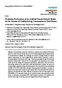
Figure 1. IRIS data distribution with respect to the sepal and petal lengths.
The optimized configuration yielded an RMS error which was reduced only marginally when the number of nodes in the hidden layer was increased further, but at the cost of a much larger computation time. It is worth mentioning here that while the number of nodes in the hidden layer used was varied from 2 for XOR to 15 for IRIS data, the number of nodes in the hidden layer was kept the same for a particular problem in different ANN algorithms to avoid any biasing towards a particular algorithm. The training of the above networks was ‘early-stopped’ to avoid any overfitting effects and this was done as soon as the RMS error reached a plateau. A maximum of ∼2000 iterations were found to be optimum for all the problems which are considered in this work. However, it is important to note that the number of iterations needed for the ANN to learn the input/output mapping depends on the complexity of the problem. In real-world problems, e.g. star/galaxy classification [6], spectra classification, primary energy estimation of Cherenkov telescopes [26] etc. ∼10,000 iterations have been used. 3.1 IRIS problem Fisher et al [27] introduced a benchmark dataset that contains the sepal and petal measurements of different types of iris flowers. There are 150 training samples available, each of which consists of four inputs and one output. The inputs are the measured lengths and widths of the petals and the sepals, and the output is the type of iris flower, such as setosa, versicolor and virginica. The distributions of the samples with respect to the dimensions of the sepals and petals are shown in 312
Pramana – J. Phys., Vol. 74, No. 2, February 2010
Comparative performance of some popular ANN algorithms Table 1. Mean RMS error and training time of various ANN algorithms with a configuration of 4 : 15 : 1 for the IRIS problem. The abbreviations used for different ANN algorithms are the following: BAC PRO – backpropagation; RES BAC – resilient backpropagation; LAV MAR – Lavenberg–Marquardt; CON GRA – conjugate gradient; RAD BAS – radial basis; SIM ANN – simulated annealing; NEU FUZ – neuro-fuzzy; HIG ORD – higher order. ANN algorithm
BAC PRO
RES BAC
LAV MAR
CON GRA
RAD BAS
SIM ANN
NEU FUZ
HIG ORD
RMS error
2.00× 10⁻³
1.75× 10⁻³
1.92× 10⁻⁵
9.64× 10⁻³
3.99× 10⁻³
1.20× 10⁻³
1.14× 10⁻³
1.21× 10⁻⁵
Time (s)
33
28
70
51
118
123
311
128
figure 1 for an easy visualization. It is quite evident from figure 1 that the classes of versicolor and virginica overlap, whereas the class of setosa is clearly separated from the other two classes. In order to convert the training data in the [0,1] interval, all measurement values were first divided by 10. The three iris species, setosa, versicolor and virginica, were categorized with the numbers 1, 2 and 3, respectively. The configuration employed for training the ANN consists of 4 : 15 : 1, i.e., 4 neurons in the input layer, 15 neurons in the hidden layer and 1 neuron in the output layer corresponding to the category of the species. The choice of 15 neurons was found to be optimum for this task. Since the final RMS error also depends upon the choice of initial parameters (like α, β and the initial weights), these parameters were changed randomly five times and final RMS error presented here is the mean of these five RMS error values. The RMS error obtained at the end of the training process for all the algorithms along with time taken for completing the training is presented in table 1. The test set for the IRIS data is similar to the training set except that these data have not been presented during the training of the nets. It consists of 45 data points (15 from each class). Instead of testing the performance of all the algorithms with test data, we have only chosen one (or sometimes two) ANN algorithm for testing purpose and these are the ones which yield the lowest RMS error during their training stage. Since for the IRIS data case both higher-order and Lavenberg–Marquardt algorithms yield the lowest (and reasonably comparable also) RMS error, we have used only these algorithms for checking their performance on the test data. The test results obtained for these algorithms suggest that while 100% classification is achievable for setosa, the classification for versicolor and virginica is only 80%. The reason for not able to obtain 100% classification between versicolor and virginica seems to be the overlapping between these two species (figure 1). 3.2 XOR and N-bit parity problems XOR is a standard and thoroughly investigated problem in the field of neural network research. Its popularity originates from the fact that, being able to solve it was Pramana – J. Phys., Vol. 74, No. 2, February 2010
313
V K Dhar et al Table 2. Mean RMS error and training time of various ANN algorithms with a configuration of 2 : 2 : 1 for the XOR problem. Full form of the abbreviations used for different ANN algorithms can be seen in the caption of table 1. ANN algorithm
BAC PRO
RES BAC
LAV MAR
CON GRA
RAD BAS
SIM ANN
NEU FUZ
HIG ORD
RMS error
1.23× 10⁻³
7.72× 10⁻³
1.59× 10⁻⁸
6.66× 10⁻⁵
2.70× 10⁻³
1.18× 10⁻⁴
2.88× 10⁻⁹
3.67× 10⁻⁷
Time (s)
16
14
15
16
18
12
15
28
a breakthrough achieved by backpropagation algorithm, compared to the situation faced when no learning algorithm was known to solve a nonlinearly separable classification task such as XOR [28]. Apart from the XOR problem we also applied other ANN algorithms to the generalized XOR problem, i.e. the N-bit parity, where the task requires to classify the sequence consisting of 1’s and 0’s according to whether number of 1’s is odd or even [28]. The target for the net here is 1 or 0 depending on whether the sequence is odd or even. In the XOR problem the algorithm used has the form 2 : 2 : 1, i.e. two neurons in the input layer, two neurons in the hidden layer and one neuron in the output layer. Also, for training the networks, more data points were also generated by incorporating random noise of 10% at the XOR inputs. The RMS error obtained for the XOR problem at the end of the training process, for all the algorithms, along with time taken for completing the training is presented in table 2. As seen from table 2, the lowest RMS error for the XOR problem is yielded by the neuro-fuzzy and the Marquardt–Lavenberg algorithms and hence performance testing on test data sample is done only for these two algorithms. Both these networks show ∼100% success rate in reproducing the XOR truth table. The parity problem too is a demanding classification task for neural networks to solve, because the target-output changes whenever a single bit in the input vector changes. The N-bit parity consists of 2N (here N = 4) training pairs. A 4 : 2 : 1 architecture was used by us for studying this problem. The RMS error obtained for the N-bit problem, at the end of the training process, for all the algorithms, along with time taken for completing the training is presented in table 3. The test set for N-bit parity problem consists of ten randomly generated noisy events (noise 10%). Testing of the net was done only with the Marquardt–Lavenberg algorithm network since compared to other algorithms considered in this work, it gives the lowest RMS error. The results obtained on the test data suggest that the 4-bit parity is reproduced with an accuracy of ∼90%. 3.3 Two-spiral problem The original two-intertwined-spiral benchmark problem was designed by Lang and Witbrock [29] to test the performance of classification on binary data. This particular task is difficult for most current algorithms since it requires the ANN model 314
Pramana – J. Phys., Vol. 74, No. 2, February 2010
Comparative performance of some popular ANN algorithms Table 3. Mean RMS error and training time of various ANN algorithms with a configuration of 4 : 2 : 1 for the 4-bit parity problem. Full form of the abbreviations used for different ANN algorithms can be seen in the caption of table 1. ANN algorithm
BAC PRO
RES BAC
LAV MAR
CON GRA
RAD BAS
SIM ANN
NEU FUZ
HIG ORD
RMS error
9.81× 10⁻⁷
7.12× 10⁻⁷
3.43× 10⁻⁸
4.03× 10⁻⁷
1.27× 10⁻⁴
9.01× 10⁻⁷
3.42× 10⁻³
5.16× 10⁻⁴
Time (s)
26
40
50
16
28
28
44
55
Table 4. Mean RMS error and training time of various ANN algorithms with a configuration of 2 : 15 : 1 for the two-spiral problem. Full form of the abbreviations used for different ANN algorithms can be seen in the caption of table 1. ANN algorithm
BAC PRO
RES BAC
LAV MAR
CON GRA
RAD BAS
SIM ANN
NEU FUZ
HIG ORD
RMS error
1.51× 10⁻¹
7.13× 10⁻¹
1.09× 10⁻¹
1.23× 10⁻¹
1.37× 10⁻¹
1.70× 10⁻¹
1.38× 10⁻¹
1.13× 10⁻¹
Time (s)
60
56
110
160
315
200
390
190
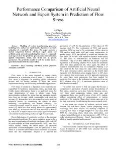
to learn the highly non-linear separation of the input space. In this benchmarking problem, two spirals, each of which has three complete turns, are created inside a unit square (figure 2). The two-intertwined-spiral problem has also been used quite extensively by other researchers as standard benchmark problem and requires the neural network to learn a mapping that distinguishes between points on two intertwined spirals. The data used by us for the 2-spiral problem contain 194 data points (97 samples per spiral). The network configuration chosen to represent this problem has the 2 : 15 : 1 architecture, where the two inputs correspond to a1 , a2 values of the two spirals and one output corresponds to whether the value belongs to the spiral 1 or spiral 2 (1 if the point falls on one spiral and 0 if it falls on the other spiral). Out of these 194 data points, 164 were used for training and 30 points (15 from each spiral) were used for testing. The training results obtained for all the ANN algorithms used in the present study are presented in table 4 and it is quite evident from this table that the Levenberg–Marquardt algorithm gives the best convergence results. However, from training time considerations, the standard backpropagation and the resilient backpropagation algorithms are seen to consume minimum training time. Performance check of the Levenberg–Marquardt algorithm, on test data for 30 points (15 from each spiral), indicates that ∼70% of the events are classified in the proper spiral category. This is much better as compared to resilient backpropagation which can classify only ∼50% of the events properly.
Pramana – J. Phys., Vol. 74, No. 2, February 2010
315
V K Dhar et al 1.0 b (2n) = 0 b(2n-1) = 1
0.9
Relevant equations for generating the spiral data are the following :
0.8 a
0.7
a
0.6
a2
(2n-1)
= 1- a1
1 (2n-1) 2
= 1-
(2n-1)
b
0.5
(2n)
a2(2n)
= r sin( α ) + 0.5 n
n
= r cos( α ) + 0.5 n
n
= 1
(2n)
b
0.4
= 0 r = 0.4 (105-n) /104 n
α =
0.3
n
π ( n -1) / 16
where n= 1,2, ......... 97
0.2 0.1 0.0 0.0
0.1
0.2
0.3
0.4
0.5
0.6
0.7
0.8
0.9
1.0
a1
Figure 2. Distribution of data points on the two interwined spirals. Table 5. Comparison of mean RMS error for different ANN algorithms considered for the study of benchmark problems. ANN algorithms Backprop Resilient Lavenberg Conjugate Rad. Basis Sim. Annealing N. Fuzzy Hig. Order
IRIS problem
XOR problem
N-bit parity
Two-spiral problem
2.00 × 10⁻³ 1.75 × 10⁻³ 1.92 × 10⁻⁵ 9.64 × 10⁻³ 3.99 × 10⁻³ 1.20 × 10⁻³ 1.14 × 10⁻³ 1.21 × 10⁻⁵
1.23 × 10⁻³ 7.72 × 10⁻³ 1.59 × 10⁻⁸ 6.66 × 10⁻⁵ 2.70 × 10⁻³ 1.18 × 10⁻⁴ 2.88 × 10⁻⁹ 3.67 × 10⁻⁷
9.81 × 10⁻⁷ 7.12 × 10⁻⁷ 3.43 × 10⁻⁸ 4.03 × 10⁻⁷ 1.27 × 10⁻⁴ 9.01 × 10⁻⁷ 3.42 × 10⁻³ 5.16 × 10⁻⁴
1.51 × 10⁻¹ 7.13 × 10⁻¹ 1.09 × 10⁻¹ 1.23 × 10⁻¹ 1.37 × 10⁻¹ 1.70 × 10⁻¹ 1.38 × 10⁻¹ 1.13 × 10⁻¹
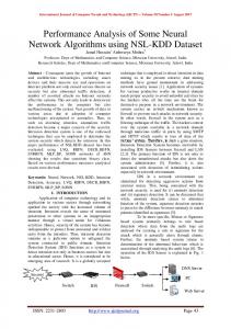
A consolidate report of the mean RMS error yielded by various ANN algorithms used in the present work for all the four benchmark problems is presented in table 5. A plot of the RMS error as a function of the number of iterations, for all the four benchmark problems is also shown in figure 3 so that the performance of the backpropagation algorithm can be compared with other algorithms. For the sake of clarity, the RMS error is shown only for the backpropagation algorithm and one more specific algorithm which yields the minimum RMS error (i.e. higherorder for IRIS, neuro-fuzzy for XOR and Levenberg–Marquardt method for Nbit parity and two-spiral problem). It is evident from figure 3 and table 5 that the Lavenberg–Marquardt method yields a lower RMS error as compared to the standard backpropagation method. Even for the IRIS and XOR problems, where 316
Pramana – J. Phys., Vol. 74, No. 2, February 2010
Comparative performance of some popular ANN algorithms 103
(a) IRIS
102 100
RMS Error
RMS Error
101 10-1 10-2
Backpropagation
10-3 10-4
Higher Order
10-5 10-6 0
500
1000
1500
102 101 100 10-1 10-2 10-3 10-4 10-5 10-6 10-7 10-8 10-9
(b) XOR
Backpropagation
Neuro Fuzzy
0
2000
1000
1500
2000
(d) 2 spiral
(c) N bit parity 101
RMS Error
RMS Error
102 101 100 10-1 10-2 10-3 10-4 10-5 10-6 10-7 10-8
500
No. of iterations
No. of iterations
Backpropagation
Levenberg
0
500
100 Backpropagation
10-1 1000
1500
No. of iterations
2000
Levenberg
0
500
1000
1500
2000
No. of iterations
Figure 3. Variation of RMS error as a function of the number of iterations for the four benchmark problems: (a) IRIS, (b) XOR, (c) N-bit parity and (d) two-spiral. The RMS error is shown only for the backpropagation algorithm and one more specific algorithm which yields the minimum RMS error for a particular problem.
higher-order and neuro-fuzzy algorithms, respectively are found to yield the lowest RMS error, the performance of the Levenberg–Marquardt algorithm is always better than the remaining ANN algorithms. The reason for the superior performance of Levenberg–Marquardt algorithm is due to the fact that it is a combination of gradient descent which is a first-order optimization algorithm and Gauss–Newton method which combines the advantages of the local convergence properties of the Gauss–Newton method and the global properties of gradient descent algorithm. However, the computational complexity of backpropagation is only O(n) as against O(n3 ) for the Levenberg–Marquardt algorithm (where n is the total number of weights in the network). 4. Application of ANN algorithms to regression problems Artificial neural networks have become a popular tool for approximating non-linear functions in higher dimensions. Although they are not the panacea for these types of problems, they are nevertheless recognized as a useful tool for approximating nonlinear functions. Other well-known methods which are conventionally used for these problems include splines [30], additive models [31], MARS [32], hinging hyperplanes Pramana – J. Phys., Vol. 74, No. 2, February 2010
317
V K Dhar et al Table 6. Mean RMS error and training time of various ANN algorithms with a configuration of 1 : 2 : 1 for the (cos(2x)+1)/3 problem. The abbreviations used for different ANN algorithms are the same as in the caption of table 1. ANN algorithm
BAC PRO
RES. BAC
LAV MAR
CON GRA
RAD BAS
SIM ANN
NEU FUZ
HIG ORD
RMS error
9.83× 10⁻⁶
7.61× 10⁻⁵
3.29× 10⁻⁷
7.30× 10⁻⁶
4.15× 10⁻⁵
4.61× 10⁻⁶
6.71× 10⁻⁶
8.12× 10⁻⁷
Time (s)
7
7
12
8
12
15
25
20
[33] and CART [34]. While none of these methods are likely to perform consistently better than the others across a wide range of problems, it is indeed a non-trivial task to develop a method that is truly effective for all types of non-linear functions. Keeping in view the superior ability of ANNs to capture non-linear behaviour of a function and its reasonably fast computation speed, we were tempted to apply the ANN as a regression tool for approximating functions like cos(x) and a few special functions like the gamma function, the complimentary error function and the upper tail cumulative χ2 -distribution function [35]. 4.1 Approximation to cos(x) To test the performance of the ANN algorithms as a regression analysis tool, we have first applied the ANN algorithms to a simple trigonometric function like y = cos(x). In order to keep the output range of the network between 0 and 1, we follow the approach given in [28] where the function is changed to y = (cos(2x) + 1)/3. The ANN configuration chosen for this problem (i.e. 1 : 2 : 1) and the number of data points used for training (=200) is again similar to that used by [28]. The training data set for this problem is synthesized by evaluating the function y = (cos(2x) + 1)/3 at 200 randomly chosen points which are picked uniformly in the interval [0, π] range (figure 4a). Additional 100 data points, following the same prescription, were also generated for testing the best ANN algorithm which produces the lowest RMS error during training. The training results obtained for all the ANN algorithms used in the present study are presented in table 6. The results of the generalization performance of the Levenberg–Marquardt algorithm, which yields the lowest RMS error during training, is shown in figure 4. In this figure, we have plotted the relative error in y (defined as (yANN − yEXP )/yEXP ) as a function of x for 100 random data points generated uniformly in the interval [0, π]. Here, for a given value of x, yANN is the value predicted by the ANN and yEXP is the expected value of the function (cos(2x) + 1)/3. It is evident from figure 4b that except for x values in the vicinity of π/2 radians, where the function y = (cos(2x) + 1)/3 itself becomes close to zero, the relative error in y is in general 0, χ2 ≥ 0, (5) 2 Γ(ν/2) χ2 where ν is the degrees of freedom. The approximation of the χ2 upper tail cumulative distribution function (Q(χ2 |ν)) was implemented with a ANN configuration of 2 : 20 : 1 where the two input nodes correspond to the χ2 and ν values. The output node of the ANN represents the (ln Q(χ2 |ν)) value. About 1000 values with 1≤ χ2 ≤ 100 and 1 ≤ ν ≤ 100 were used for training the ANN algorithms. The training of the ANN was performed with only those values of χ2 and ν which yield a (Q(χ2 |ν)) between ∼1.757 × 10⁻²³ and 0.999. The results of the training regarding the mean error for all the three special functions discussed above are presented in table 7. Performance of the Levenberg–Marquardt algorithm in terms of relative error in approximating the three special functions is shown in figure 5. A data sample of 100 values each is used for testing the approximation for the gamma function (figure 5a) and Gaussian upper tail probability integral (figure 5b). The corresponding data samples used for testing the χ2 upper tail probability integral is 400 for four different values of ν. Referring first to the approximation of the gamma function, it is evident from figure 5a that the relative error in Γ(z) is