Forests 2015, 6, 3704-3732; doi:10.3390/f6103704 OPEN ACCESS
forests ISSN 1999-4907 www.mdpi.com/journal/forests Article
Comparing ALS and Image-Based Point Cloud Metrics and Modelled Forest Inventory Attributes in a Complex Coastal Forest Environment Joanne C. White 1,*, Christoph Stepper 2, Piotr Tompalski 3, Nicholas C. Coops 3 and Michael A. Wulder 1 1
2
3
Canadian Forest Service, Natural Resources Canada, 506 West Burnside Road, Victoria, BC V8Z 1M5, Canada; E-Mail:
[email protected] Bavarian State Institute of Forestry (LWF), Department of Information Technology, Research Group: Remote Sensing, Hans-Carl-von-Carlowitz-Platz 1, Freising D-85354, Germany; E-Mail:
[email protected] Department of Forest Resources Management, Forest Science Centre, 2424 Main Mall, University of British Columbia, Vancouver, BC V6T 1Z4, Canada; E-Mails:
[email protected] (P.T.);
[email protected] (N.C.C.)
* Author to whom correspondence should be addressed; E-Mail:
[email protected]; Tel.: +1-250-298-2402; Fax: +1-250-363-0775. Academic Editor: Eric J. Jokela Received: 4 August 2015 / Accepted: 8 October 2015 / Published: 15 October 2015
Abstract: Digital aerial photogrammetry (DAP) is emerging as an alternate data source to airborne laser scanning (ALS) data for three-dimensional characterization of forest structure. In this study we compare point cloud metrics and plot-level model estimates derived from ALS data and an image-based point cloud generated using semi-global matching (SGM) for a complex, coastal forest in western Canada. Plot-level estimates of Lorey’s mean height (H), basal area (G), and gross volume (V) were modelled using an area-based approach. Metrics and model outcomes were evaluated across a series of strata defined by slope and canopy cover, as well as by image acquisition date. We found statistically significant differences between ALS and SGM metrics for all strata for five of the eight metrics we used for model development. We also found that the similarity between metrics from the two data sources generally increased with increasing canopy cover, particularly for upper canopy metrics, whereas trends across slope classes were less consistent. Model outcomes from ALS and SGM were comparable. We found the greatest
Forests 2015, 6
3705
difference in model outcomes was for H (ΔRMSE% = 5.04%). By comparison, ΔRMSE% was 2.33% for G and 3.63% for V. We did not discern any corresponding trends in model outcomes across slope and canopy cover strata, or associated with different image acquisition dates. Keywords: digital aerial images; image matching; airborne laser scanning; forest inventory; photogrammetry; lidar
1. Introduction Airborne laser scanning (ALS) is now widely acknowledged as an important data source for forest inventories [1]. The three-dimensional information conferred by ALS data enables the characterization of vertical forest structure, and thereby, the estimation of forest inventory attributes of interest such as height, basal area, and volume, among others [2]. Recently, digital aerial photogrammetry (DAP) has emerged as an alternative data source to ALS for three-dimensional characterization of forests [3]. Herein, we use the term DAP to encompass the range of image-based outputs derived from digital air photos that are being used to capture forest structural information, including both image-based point clouds [3], and image-derived, raster-based digital surface models (DSM) [4]. Earlier studies examining the capabilities of DAP in an area-based approach (ABA) to model forest attributes were conducted in highly managed and relatively simple forest environments (i.e., even-aged, single-layer forests) [4–7]. These studies generally found that DAP outputs could produce area-based predictive models for inventory attributes that had accuracies similar to predictive models generated using ALS data. Subsequent studies conducted in more complex forest environments (i.e., multi-aged, multi-layered) have reached similar conclusions [8,9]. Interest in image-based point clouds continues to grow with the increasing availability of appropriate digital imagery with improved radiometric and geometric properties. In many jurisdictions in Europe, digital aerial imagery are routinely acquired and updated by national mapping agencies [10], and many of these same jurisdictions also have high quality digital terrain models derived from ALS data [3]. Forestry is a discipline with a long history of utilizing aerial photography to inform inventory programs [11], therefore it is logical that there would be great interest in exploiting imagery (via image-based point clouds or DSM) to generate an ALS-like characterization of vegetation three-dimensional structure at a fraction of the cost [3]. Whereas the widespread use of ALS data have been matched with certain standards and conventions such as the LAS file format [12], no similar conventions exist for image-based point clouds. Moreover, there are a number of different algorithms and image-matching software tools available for generating image-based point clouds. Stepper et al. [8] called for a rigorous benchmarking of image matching methods for forest environments, as to-date, benchmarking has only been done for non-forest targets (e.g., [13,14]). The quality and suitability of digital imagery that is being used for image matching and point cloud generation also varies. Although minimum specifications for suitable imagery have been suggested [8,15], there is little empirical data to support these specifications in terms of their impact on area-based modelled outcomes for forest inventory. Less optimal imagery (i.e., below minimum specification) is
Forests 2015, 6
3706
actively and opportunistically being used to generate image-based point clouds (e.g., [8,16]) with minimal impact on model outcomes quantified thus far [7]. Moreover, the profusion of image-matching algorithms and variability in image input data make it more difficult to compare model outcomes for existing studies in the scientific literature. This difficulty is further complicated by the fact that most studies focus on model outcomes exclusively, and do not provide a full interrogation of point cloud metrics, or at a minimum, convey some sense of the discrepancies between the ALS and image-derived point clouds (and that may be unique to the forest environment in question). An exception to this is Vastaranta et al. [6], who provide a full exploration of metrics and link model outcomes to variations in metric values. Such a comparison enabled improved understanding of the differences in how ALS and DAP characterize canopy vertical structure [3]. In addition studies that directly compare and report ALS- and DAP-based model outcomes are valuable (Table 1). Gobakken et al. [17] indicate that large-area operational scale implementation of DAP for an area-based approach may be difficult as a result of the impact that variable acquisition conditions (i.e., sun angle, light, growing season) may have on model outcomes. To our knowledge, the actual impact of varying acquisition conditions have yet to be tested and reported in the literature. Table 1. Results of selected studies that explicitly compare airborne laser scanning (ALS) and digital aerial photogrammetry (DAP) outcomes using the same modelling approaches and calibration/validation data. Vastaranta et al.,
Straub et al.,
2013 [4] ALS Study
2013 [9] DAP
Southern, Finland
location
ALS
DAP
Bavaria, Germany
Rahlf et al., 2014 [18] ALS
DAP
Southeastern, Norway
Pitt et al., 2014 [19] ALS
DAP
Gobakken et al., 2015 [17] ALS
DAP
Central Ontario,
Southeastern,
Canada
Norway
Picea mariana Dominant tree species
Pinus sylvestris, L.;
Picea abies;
Picea abies (L.)
Fagus sylvatica L.;
H. Karst.
Abies alba Mill.; mixed
Picea abies, also Pinus sylvestris
(Mill.) Britton, Sterns & Poggenb. Pinus banksiana
Picea abies, Pinus sylvestris
Lamb.; mixed Attribute Height [m]
Mean height
bias
−0.03
−0.07
bias%
−0.16
−0.35
Top height
RMSE
1.47
2.13
1.05
1.55
RMSE%
7.75
11.18
7.30
10.80
5.10
5.66
25.40
28.10
bias
0.09
0.08
Basal area
bias%
0.39
0.37
[m2·ha−1]
RMSE
3.65
4.86
RMSE%
17.76
23.62
Attribute
Total stem volume
8.68
10.14
30.21
35.29
Gross merchantable
Total stem
Gross merchantable
volume
volume
volume
Volume
bias
0.49
0.42
[m3·ha−1]
bias%
0.26
0.22
RMSE
33.64
46.1
102.78
121.99
36.20
58.59
28.14
28.71
RMSE%
17.92
24.50
31.92
37.89
19.42
31.43
26.20
26.80
Lorey’s mean height
7.5
10.2
15.4
18.3
Total volume
18.0
21.7
Forests 2015, 6
3707
In this study, we compared ALS and image-based data in the context of natural forest stands in a complex coastal forest ecosystem in western Canada. This represents an environment that heretofore has not been the subject of such comparisons, and that represents certain challenges for both ALS and imagery with its potential for dense canopy cover and steep, rugged terrain. Our first objective was to fully characterize differences between ALS- and image-based point cloud metrics across a range of environmental conditions, defined by topographic slope and canopy cover. Our second objective was to generate area-based plot-level predictive models of Lorey’s mean height, basal area, and gross volume from both sources of point cloud data and compare model outcomes in the context of the differences we observed in the ALS and DAP-derived metrics and in the context of different acquisition conditions for the imagery. 2. Materials and Methods 2.1. Study Area Our study area covers approximately 52,000 ha and is located on northern Vancouver Island, BC, Canada (Figure 1). The major tree species found within the coastal temperate rainforests in this area are western hemlock (Tsuga heterophylla (Raf.) Sarg.), western red cedar (Thuja plicata Donn ex D. Don), and amabilis fir (Abies amabilis Douglas ex J. Forbes). Other tree species found in the study area include Douglas-fir (Pseudotsuga menziesii (Mirb.) Franco), red alder (Alnus rubra Bong.), yellow cedar (Chamaecyparis nootkatensis (D.Don) Spach), mountain hemlock (Tsuga mertensiana (Bong.) Carrière), and Sitka spruce (Picea sitchensis (Bong.) Carrière). Located primarily within the wetter Coastal Western Hemlock biogeoclimatic zone (CWH), the study area is characterized by high annual precipitation (3000–5000 mm), mild winters (average temperature 0 °C to 2 °C), and cool summers (average temperature 18 °C to 20 °C) [20]. Topography strongly influences local variations in climate, with topography more extreme in the southern portion of the study area. Elevation within the study area ranges from sea level to 1200 m, with an average slope of 23.6°(standard deviation = 13.8°), and average canopy cover was 74.8% (standard deviation = 32.1%). The average age of stands was 144 years (standard deviation = 127 years).
Forests 2015, 6
3708
Figure 1. Map of the study area. (a) Location in British Columbia, Canada; (b) location on Northern Vancouver Island; and (c) boundaries of the study area units (WFP1, WFP2, and WFP3). 2.2. Ground Plot Data Given that the area-based approach requires response data that covers the full range of structural variability in the forest of interest [21,22] and moreover, given that non-parametric regression methods cannot extrapolate beyond the range of calibration data used to build the model [23], a stratified random sampling design was used to select ground plot locations in this study area. Five initial strata were defined using species information, biogeoclimatic data [20], and elevation data: (1) forests in the CWHvh1 subzone (a very wet hypermaritime subzone within CWH [20]) dominated by western red cedar; (2) low-elevation forests dominated by western hemlock and western red cedar; (3) high-elevation forests dominated by western hemlock and western red cedar; (4) high-elevation forests dominated by mountain hemlock; and (5) deciduous-leading forests. Strata 1–3 accounted for approximately 94% of the study area. A total of 140 ground plots were established, with 85% of plots allocated to the first three strata, and the remainder allocated to the last two strata. Within each stratum, sample locations were selected by a systematic partition of the three-dimensional ALS-derived feature space, as defined by the 80th percentile of ALS heights, the coefficient of variation of ALS heights, and canopy density. In the field, plot centres were established with a Trimble GeoXH GPS receiver equipped with an external Tornado antenna. On average, more than 900 GPS
Forests 2015, 6
3709
measures were acquired per plot centre. Plot positions were differentially corrected to have sub-metre planimetric precision. Plots were circular in shape, with a radius of 14 m and an area of 615.75 m2. Within each plot, all live standing trees with diameter at breast height (dbh) ≥12.0 cm were measured. Individual tree measures included dbh (cm), stem height (m), species, age, and other mensurational data. Individual tree-based estimates of stem height and diameter were used to compute estimates of Lorey’s mean height (m), basal area (m2·ha−1), and gross volume (m3·ha−1). Ground plot characteristics for Lorey’s mean height (H), basal area (G), and gross volume (V), are summarized in Table 2 and Figure 2. Table 2. Summary of ground plot characteristics (n = 140).
Lorey’s mean height (m) Basal area (m2 ha−1) Gross volume (m3 ha−1)
Minimum
1st Quartile
Median
3rd Quartile
Maximum
Mean
Standard Deviation
8.6
24.9
32.1
40.0
54.7
32.1
10.2
3.3
49.7
66.5
90.7
154.9
70.7
32.6
15.3
554.4
897
1261.3
2,481.9
940.3
530.7
Figure 2. Boxplots showing the variability of the ground plots characteristics Lorey’s mean height, basal area, and gross volume (n = 140). 2.3. ALS Data ALS point clouds were acquired in August and September of 2012 using an Optech ALTM3100EA scanning system (Table 3) operated at an altitude of approximately 700 m above ground level. The average return point density was 11.6 points/m2. A Digital Terrain Model (DTM) with a spatial resolution of 1 m was created using ground returns and standard pre-processing routines as per Axelsson (2000) [24]. The DTM was then used to normalize ALS point cloud heights to heights above ground level.
Forests 2015, 6
3710 Table 3. ALS data acquisition specifications and characteristics. Parameter Sensor Aircraft Speed Data Acquisition Height Swath width Max scan angle Beam divergence Wavelength Overlap Pulse Repetition Rate Scan Frequency Number of Returns Per Pulse Point Density
Description ALTM3100EA 240 km/h 700 m AGL 323 m 25° 0.3 mrad 1064 nm 75% 70 KHz 65 Hz 4 11.6 pt./m2
2.4. Digital Aerial Imagery Digital imagery was acquired for the study area using a Vexcel UltraCamX camera (Table 4). Due to the size of the area of interest, topographic complexity, and variable acquisition conditions (i.e., fog, low cloud), complete coverage of the study area was achieved through separate flights on 16 August, 25 September, and 4 and 6 October of 2012. Of note, the average sun elevation in the study area associated with each of those dates was 42.5°, 36.5°, 33.8°, and 33.1°, respectively. The imagery was 4-band (RGB and NIR) with a 0.30 m ground sampling distance. Imagery was acquired with a minimum 60% along-track and 20% across-track overlap, resulting in a total of 383 stereo images. We used the semi-global matching (SGM) algorithm [25] to generate dense image-based point clouds, implemented in the Remote Sensing Software Package Graz (RSG version 7.46.11) [26]. Processing was conducted separately for each of the three sub-areas identified in Figure 1c. Given the low across-track overlap of the images, only along-track stereo pairs were used for matching, as per Stepper et al. [8]. The resulting point density of the image-based point cloud was 12.27 points/m2. To achieve heights above ground, the image-based points were normalized by subtracting the ALS-based terrain heights. Table 4. Digital aerial image acquisition specifications and characteristics. Parameter Sensor Data Acquisition Height Across-track overlap Along-track overlap GSD Cross-track field of view Along-track field of view Pixel size Point Density
Description UltraCamX 4,187 m AGL 20% 60% minimum 0.30 m 55° 37° 7.2 μm 12.27 pt./m2
Forests 2015, 6
3711
2.5. Metric Generation and Comparison In order to thoroughly evaluate differences between ALS and SGM metrics, we conducted a comparison of the derived point cloud metrics across the range of topographic slope and canopy cover conditions existing within the study area (Table 5). To enable this comparison, we tessellated our study area into 25 m by 25 m raster cells. For each raster cell we computed slope (in degrees) from the ALS DTM and canopy cover from the normalized ALS point cloud. Canopy cover was determined as the proportion of ALS points >2 m for 25 m by 25 m raster cells across the study area. We then defined 16 strata through a combination of slope and canopy cover conditions (Table 5). We applied a negative buffer of 25 m (one cell width) to all cells having the same stratum in order to avoid selection of adjacent cells for analysis. Within the buffered zones, we then randomly selected 50 sample cells from each stratum (Table 5), resulting in a total of 797 sample cells (two strata did not yield 50 samples). For all of the selected raster cells, the standard suite of ALS height and density metrics were generated from the normalized ALS and SGM point clouds using the FUSION cloudmetrics function and a lower threshold of 2 m and an upper threshold of 100 m (version 3.42) [27]. Table 5. Slope and canopy cover class strata. The number of sample raster cells (25 m by 25 m) within each stratum is indicated. The numbers in parentheses indicate the number of corresponding ground samples within each stratum; while n indicates the stratum number (for cross-referencing to Tables 7, 8, and 11). Slope (°) 0–5 5–20 20–30 ≥30 Total
0–10 50 (0); n = 11 50 (0); n = 21 50 (0); n = 31 48 (0); n = 41 198
10–50 50 (1); n = 12 50 (0); n = 22 50 (0); n = 32 49 (0); n = 42 199
Cover (%) 50–90 50 (2); n = 13 50 (14); n = 23 50 (5); n = 33 50 (9); n = 43 200
90–100 50 (12); n = 14 50 (37); n = 24 50 (32); n = 34 50 (28); n = 44 200
Total 200 200 200 197 797
To enable comparisons between ALS and SGM metrics and assess their agreement, for each stratum we calculated the mean difference (MD) and the root mean squared deviation (RMSD) between the ALS and SGM metrics using Equations (1) and (2). RMSD indicates the average difference between metric values for each stratum, and informs on the magnitude of the differences between the ALS and SGM metric values, whereas MD indicates whether the SGM metrics are generally greater or less than the corresponding ALS metric values. We calculated the Spearman rank correlation coefficient (denoted as r) between ALS and SGM metric values for each stratum to assess the degree of association between metric values. Finally, we used a Wilcoxon matched pairs test to evaluate whether the differences between metric median values were statistically significant.
Forests 2015, 6
3712 𝑛
1 𝑀𝐷 = ∑(𝑆𝐺𝑀𝑖 − 𝐴𝐿𝑆𝑖 ) 𝑛
(1)
𝑖=1
𝑛
1 𝑅𝑀𝑆𝐷 = √ ∑(𝑆𝐺𝑀𝑖 − 𝐴𝐿𝑆𝑖 )2 𝑛
(2)
𝑖=1
Subsequent modelling of our inventory attributes of interest was enabled by generating height and density metrics for the ALS and SGM point clouds corresponding to our 140 ground plot locations. ALS and SGM point clouds were clipped to the spatial extent of the ground plots (i.e., circular with a radius of 14 m) for metric generation. The same suite of ALS height and density metrics as were generated for our sample raster cells above, were also generated for these clipped point clouds using the FUSION cloudmetrics function. Thus we had two datasets to support our subsequent analyses: a set of ALS and SGM metrics for 25 m by 25 m raster cells (n = 797) distributed across a range of slope and canopy cover conditions within our study area that we used to support a detailed assessment of metric characteristics; and a set of plot-based metrics (n = 140) that were used for area-based modelling of forest inventory attributes. 2.6. Area-Based Modelling of Forest Attributes An ensemble regression tree algorithm, Random Forests (RF) [28], was used to model H, G, and V. RF was implemented using the R packages caret [29] and randomForest [30,31]. In order to achieve parsimonious models, we selected a subset of metrics to be used as predictor variables in our RF models (Table 6). The selection of these metrics was informed by the scientific literature, and also by our experiences in modeling these attributes across a range of forest environments [32,33]. For validation of model outcomes, we applied a 10-fold cross-validation repeated five times as recommended by Kuhn and Johnson [34]. Thus, in total, 50 different hold-out datasets (referred to as folds, f) were used to assess the model performance for H, G, and V. Table 6. Metrics calculated from the ALS and semi-global matching (SGM) point clouds that were used for metric comparison across the different strata and as inputs to the Random Forests models. Metric Hmean CoV Skewness Kurtosis P10 P90 CCmean Rumple
Description Average of point heights >2 m Coefficient of variation of point heights >2 m Skewness of point heights >2 m Kurtosis of point heights >2 m 10th percentile of point heights >2 m 90th percentile of point heights >2 m Percentage of point heights >mean height Ratio of three-dimensional canopy surface model area to ground area
For all folds, the root mean squared error (RMSE) and bias were calculated (Equations (3) and (4)). In order to get overall measures of the models’ precision and accuracy, the obtained 𝑅𝑀𝑆𝐸𝑓 - and 𝑏𝑖𝑎𝑠𝑓 values were averaged over the 50 separate folds. These measures correspond to the repeated
Forests 2015, 6
3713
cross-validation estimates of model performance (Equations (5) to (8)). In these equations, 𝑦𝑖 is the observed value, 𝑦̂𝑖 is the predicted value for the 𝑖th of 𝑛 sample plots in one of the 𝑘 held-out sets, and 𝑦𝑓 is the mean of 𝑛 observed values in that hold-out set. ∑n𝑖=1(𝑦𝑖 − 𝑦̂𝑖 )2 n
𝑅𝑀𝑆𝐸𝑓 = √
∑n𝑖=1(𝑦𝑖 − 𝑦̂𝑖 ) 𝑏𝑖𝑎𝑠𝑓 = n RMSE = RMSE% =
bias = bias% =
∑𝑘𝑗=1 𝑅𝑀𝑆𝐸𝑓,𝑗 𝑘 RMSE × 100 mean(𝑦̅𝑓 ) ∑𝑘𝑗=1 𝑏𝑖𝑎𝑠𝑓,𝑗 k bias × 100 mean(𝑦̅𝑓 )
(3)
(4)
(5)
(6)
(7)
(8)
In order to relate the differences observed between the ALS and SGM metrics across our strata of slope and canopy cover classes to the model outcomes, we identified strata membership for each of our 140 plots (Figure 3 and Table 5) and calculated relative model RMSE and bias, by stratum. We likewise determined the corresponding image acquisition date associated with each of our plots, and calculated relative model RMSE and bias by acquisition date. We used a paired t-test to evaluate whether the mean values of the differences between the ground plot data and the predicted values (for bias) or the mean of the squared differences (for RMSE) for ALS and SGM predictions were significantly different.
Forests 2015, 6
3714
Figure 3. Distribution of slope (°) and canopy cover (%) across the study area. (a) Histogram of slope; (b) histogram of canopy cover; (c) hexagonal binning of all 25m by 25m cells within the study area. Superimposed are the locations of the 797 sample cells and the 140 ground plots with respect to the prevailing slope and canopy cover. The dashed lines indicate the strata boundaries (cf. Table 5). 3. Results 3.1. Metric Comparison ALS and SGM metrics used for attribute models were compared across the 16 strata defined by ALS-derived slope and canopy cover (Table 5, Figures 3 and 4). Trends across our sampled strata (Table 7) vary by metric, but some common themes emerge. For example, by examining the 90th percentile of heights (P90), it is evident that the P90SGM is generally greater than the P90ALS (indicated by positive MD values, with mean value for all strata = 2.21 m) and that the difference between them, as indicated by the RMSD (mean = 4.37 m), generally decreases with increasing canopy cover (Figure 5). On average, the P90SGM is 4.88 m higher than the corresponding ALS value for canopy
Forests 2015, 6
3715
cover of 0%–10%. By comparison, the P90SGM is only 0.66 m higher when canopy cover is 90%–100%. Similarly, correlation between P90ALS and P90SGM increases with increasing canopy cover, from a mean r = 0.13 for canopy cover of 0%–10%, to a mean r = 0.94 for canopy cover of 90%–100%. Regarding the trends across slope gradients, both MD and RMSD for P90 increase on average with increasing slope (mean MD = 1.40 m for slope 0°–5°, mean MD = 4.05 m for slope 30°–90°; mean RMSD = 3.24 m for slope 0°–5°, mean RMSD = 7.20 m for slope ≥30°). In contrast, the correlation between P90SGM and P90ALS appears to be relatively independent of the prevailing slope condition. Of note, P90 was the one metric for which there was no statistically significant difference between SGM and ALS median values for several of the strata, primarily for those with ≥50% canopy cover (Table 8). For mean height (Hmean), MDs across all strata are generally larger than for P90 (mean MD for Hmean = 3.26 m), whereas the averaged RMSD of 4.36 m is almost equal to that of the P90. Examining the different canopy cover classes (Figure 6) indicates that strong correlations (i.e., |r| ≥ 0.8) between ALS and SGM Hmean occur for canopy cover ≥50%. The average MD for Hmean is 4.38 m for canopy cover 50%–90% and 3.79 m for strata with canopy cover 90%–100%. The corresponding RMSDs are 5.72 m and 5.26 m, respectively. Examining only those strata with canopy cover ≥50%, the scatterplots in Figure 6 reveal a decreasing correspondence between the SGM and ALS Hmean with increasing slope. This is particularly evident at slopes ≥30°, with MD and RMSD of 7.15 m and 9.28 m (mean of strata 43 and 44), respectively, compared to 3.08 m and 4.23 m for the less steep strata (mean of strata 13, 14, 23, 24, 33, 34). The differences between SGM and ALS Hmean metric medians were significant across all strata (Table 8). When examining the 10th percentile of heights (P10), it is evident that there is greater disparity between SGM and ALS metric values. Of note, MD and RMSD are very large for P10, particularly for high canopy cover and steep slopes (Figure 7), and SGM and ALS median metric values are significantly different for all strata (Table 8). Trends for other metrics vary. The coefficient of variation of point heights (CoV) is consistently smaller for SGM data across all strata (i.e., MD is always negative), indicative of the different canopy penetration capacity of the SGM relative to the ALS data. Values for the SGM skewness metric are likewise smaller than their ALS counterparts, except for strata with canopy cover >90% (i.e., 14, 24, 34, 44). SGM kurtosis values tend to be lower than their ALS counterparts, except for strata with 50%–90% canopy cover.
Forests 2015, 6
Figure 4. Selected comparison of ALS and SGM point clouds for the same cell locations across the range of slope and canopy cover conditions, as described in Table 5. Metrics P90, P10, CCmean, and Rumple are defined in Table 6.
3716
Forests 2015, 6
3717
Table 7. Results of metric comparisons across strata defined in Table 5. Mean Difference (MD) and Root Mean Squared Difference (RMSD) are calculated using Equations (1) and (2), respectively. Spearman rank order correlations (r) are reported between ALS and SGM metrics. Values in italics are significant at p < 0.05. Metrics are defined in Table 6. Hmean
CoV
Skewness
Kurtosis
STRATUM
MD
RMSD
r
MD
RMSD
r
MD
RMSD
R
MD
RMSD
r
11
2.69
3.44
0.01
−0.07
0.50
0.21
−0.89
2.20
0.00
−6.89
19.47
−0.16
12
1.34
1.61
0.71
−0.62
0.69
0.04
−0.91
1.10
0.17
−2.38
3.98
0.08
13
3.01
3.73
0.75
−0.40
0.41
0.64
−0.45
0.58
0.60
0.34
1.20
0.05
14
2.34
3.37
0.95
−0.20
0.24
0.00
1.25
1.42
0.36
−1.03
2.85
0.09
21
2.34
2.81
0.10
−0.12
0.34
−0.35
−0.80
1.81
−0.26
−3.52
11.83
−0.19
22
1.31
1.95
0.16
−0.27
0.43
0.32
−0.36
1.00
0.30
0.00
4.98
0.37
23
2.42
3.22
0.84
−0.36
0.40
0.28
−0.28
0.60
0.31
0.69
1.49
−0.14
24
3.02
3.93
0.97
−0.19
0.21
0.36
1.03
1.30
0.11
−1.14
2.62
0.18
31
2.39
2.79
0.14
−0.21
0.39
0.14
−1.43
3.88
0.09
−21.36
123.72
0.01
32
1.43
2.40
0.17
−0.18
0.41
0.38
−0.48
1.18
0.29
−0.14
6.60
0.15
33
4.67
6.30
0.93
−0.27
0.42
0.17
−0.16
0.62
0.51
0.64
1.47
−0.08
34
3.03
4.84
0.89
−0.18
0.22
−0.03
1.09
1.30
0.13
−1.30
2.44
0.04
41
3.71
4.32
0.27
−0.24
0.34
0.05
−1.25
1.69
0.15
−6.89
17.60
0.14
42
4.16
6.50
0.41
−0.47
0.79
−0.03
−1.01
1.51
0.19
−3.88
13.48
0.22
43
7.49
9.64
0.78
−0.37
0.45
0.04
−0.24
0.66
0.29
0.47
2.66
0.29
44
6.80
8.91
0.87
−0.23
0.29
0.15
0.52
0.80
0.34
−0.23
0.99
0.37
Mean
3.26
4.36
0.56
−0.27
0.41
0.15
−0.27
1.35
0.22
−2.91
13.59
0.09
P10
P90
CCmean
Rumple
STRATUM
MD
RMSD
r
MD
RMSD
r
MD
RMSD
r
MD
RMSD
r
11
0.55
0.87
0.01
5.09
6.40
0.00
22.83
29.04
0.10
−4.89
37.18
−0.20
12
0.43
0.55
0.36
0.63
1.76
0.68
15.28
17.06
0.01
−0.67
0.99
0.70
13
3.74
5.03
0.13
0.13
2.67
0.75
5.15
6.75
0.47
−0.92
1.37
−0.06
14
9.46
12.50
−0.14
−0.27
2.14
0.96
−12.20
14.71
−0.02
−0.26
0.89
0.59
21
0.48
0.74
−0.31
4.61
5.55
0.21
9.54
14.97
−0.37
5.24
20.01
0.14
22
0.48
0.86
0.32
1.63
3.27
0.08
8.82
12.99
0.12
0.20
0.89
0.16
23
3.28
4.24
−0.08
0.09
1.96
0.90
4.98
7.21
0.27
−0.94
1.26
0.54
24
8.65
11.38
0.28
0.04
1.91
0.98
−7.30
9.39
0.15
−0.57
0.96
0.56
31
0.98
1.42
0.28
4.01
4.73
0.12
10.17
13.88
−0.01
2.85
14.17
−0.04
32
1.07
1.94
0.28
1.15
3.95
0.12
6.35
10.18
0.32
1.86
14.07
0.33
33
7.77
10.99
−0.63
1.46
3.58
0.95
2.46
8.05
0.35
−1.42
1.97
0.67
34
8.07
11.53
0.14
0.60
3.27
0.92
−8.26
10.53
0.03
−0.32
1.09
0.48
41
1.82
2.50
0.30
5.83
6.66
0.20
11.57
14.62
−0.08
3.33
14.53
0.08
42
3.01
5.18
−0.15
4.65
9.70
0.45
11.97
17.28
0.09
3.91
19.53
0.50
43
10.97
13.86
−0.07
3.43
6.91
0.83
3.63
8.62
0.15
−1.51
2.19
0.32
44
14.23
17.29
0.01
2.29
5.55
0.89
−5.56
8.49
0.32
−0.90
1.73
0.54
Mean
4.69
6.30
0.05
2.21
4.37
0.56
4.96
12.73
0.12
0.31
8.30
0.33
Forests 2015, 6
3718
Figure 5. Scatterplots of ALS and SGM 90th percentiles of height (P90) metrics across the strata defined by slope and canopy cover classes. Table 8. Results of Wilcoxon matched pairs test for statistical significance of the differences between the metric medians from SGM and ALS point cloud data at p < 0.05. Metric Hmean CoV Skewness Kurtosis P10 P90 CCmean Rumple
Number of Strata with No Significant Differences 0 1 0 0 0 5 0 2
Stratum with No Significant Difference 11
13, 14, 23, 24, 34 22, 42
Forests 2015, 6
Figure 6. Scatterplots of ALS and SGM mean height (Hmean) metrics across the strata defined by slope and canopy cover classes.
3719
Forests 2015, 6
3720
Figure 7. Scatterplots of ALS and SGM 10th percentiles of height (P10) across the strata defined by slope and canopy cover classes. For the canopy cover metric (CCmean, the proportion of point heights greater than the mean point height), the r values are generally low, indicating that there is not a strong correlation between the SGM and ALS CCmean. The MD generally decreased with increasing canopy cover, except for strata with canopy cover >90%. CCmeanSGM overestimates canopy cover relative to CCmeanALS by an average of 13.53% for strata with canopy cover of 0%–10%, and conversely, CCmeanSGM underestimates cover relative to CCmeanALS by an average of 8.33% for strata with canopy cover of 90%–100% (Table 7). The RMSD values are lowest for strata with canopy cover of 50%–90%
Forests 2015, 6
3721
(mean = 7.66%), and increase both for higher and lower canopy cover. Examining the different slope scenarios, no consistent pattern in CCmean was found. For Rumple, a measure of the canopy surface roughness, the MD values indicate that the SGM Rumple metric values are greater than ALS counterparts for low cover scenarios (except for slopes 0°–5°), and lower than ALS for high cover scenarios. The high RMSD values for the low cover strata (mean RMSD = 21.47 for canopy cover 0%–10%) in conjunction with the correlation being almost zero (mean r = 0.02 for canopy cover 0%–10%) point to the great discrepancy for Rumple at low canopy cover (Table 7). For the densely covered samples (canopy cover 90%–100%), the RMSD = 1.17 on average and r = 0.54, indicating a higher level of correspondence for the SGM and ALS based canopy surface at high canopy covers. Correlations between the input metrics used for model development and the plot-based estimates of H, G, and V are summarized in Table 9. For the ALS data, the metrics that were most strongly correlated with Lorey’s mean height were P90 (r = 0.96), Hmean (r = 0.88) and Rumple (r = 0.76). For the SGM data, Hmean (r = 0.91) and P90 (r = 0.90) had the strongest correlation with Lorey’s mean height (Figure 8). Of note, P10SGM—which was an average of 14.33 m greater than P10ALS for the plot data (n = 140)—was also strongly correlated with Lorey’s mean height (r = 0.88), in contrast to P10ALS (r = 0.18). Recall that for the sample cells, which covered a much broader range of forest conditions and included canopy cover