Comparing data mining and deterministic pedology to ...

Geoderma 237–238 (2015) 237–245

Contents lists available at ScienceDirect

Geoderma journal homepage: www.elsevier.com/locate/geoderma

Comparing data mining and deterministic pedology to assess the frequency of WRB reference soil groups in the legend of small scale maps Romina Lorenzetti ⁎, Roberto Barbetti, Maria Fantappiè, Giovanni L'Abate, Edoardo A.C. Costantini Consiglio per la ricerca e la sperimentazione in agricoltura, CRA-ABP Agrobiology and Pedology Research Center, Florence, Italy

a r t i c l e

i n f o

Article history: Received 10 February 2014 Received in revised form 18 July 2014 Accepted 4 September 2014 Available online xxxx Keywords: Learning machine Bayesian predictivity Soil classification Geomatic Italy

a b s t r a c t The assessment of class frequency in soil map legends is affected by uncertainty, especially at small scales where generalization is greater. The aim of this study was to test the hypothesis that data mining techniques provide better estimation of class frequency than traditional deterministic pedology in a national soil map. In the 1:5,000,000 map of Italian soil regions, the soil classes are the WRB reference soil groups (RSGs). Different data mining techniques, namely neural networks, random forests, boosted tree, classification and regression tree, and supported vector machine (SVM), were tested and the last one gave the best RSG predictions using selected auxiliary variables and 22,015 classified soil profiles. The five most frequent RSGs resulting from the two approaches were compared. The outcomes were validated with a Bayesian approach applied to a subset of 10% of geographically representative profiles, which were kept out before data processing. The validation provided the values of both positive and negative prediction abilities. The most frequent classes were equally predicted by the two methods, which differed however from the forecast of the other classes. The Bayesian validation indicated that the SVM method was more reliable than the deterministic pedological approach and that both approaches were more confident in predicting the absence rather than the presence of a soil type. © 2014 Elsevier B.V. All rights reserved.

1. Introduction Soils vary in a rather complex manner across the landscape. Therefore, attribution of soil types to a map unit is always affected by some degree of uncertainty. The level of complexity and uncertainty of soil information within map units often increase as the map scale decreases, and this can bias or lower the confidence in interpretations (Kros et al., 1999). Considerable information may be lost due to map generalization and the results can only be considered rough estimates (Ibañez et al., 1998). Nevertheless, small scale maps are very important since they play a specific role in synthesizing soil information and representing a first partition of the soilscape, allowing comparisons on a broad scale and between disciplines (Ibañez and Feoli, 2013). The traditional deterministic approach (DA) considers soil cover as partitioned into discontinuous patches of discrete classes (Soil Survey Division Staff, 1993). The mapper delineates soilscapes with relatively homogeneous expressions of soil-forming processes at the reference scale (Jenny, 1941, 1980). According to the guidelines for soil mapping provided by different systems, such as the Soil Survey Manual (Soil Survey Division Staff, 1993) and the WRB (IUSS working group WRB, 2014), soil types are classified as “dominant”, “co-dominant” and “associated” depending on their estimated coverage in the polygon. The estimate can be based on expert judgment, field surveys, image analysis of ⁎ Corresponding author.

http://dx.doi.org/10.1016/j.geoderma.2014.09.006 0016-7061/© 2014 Elsevier B.V. All rights reserved.

aerial photographs or satellite images, by attribution of similar soils to similar soilscapes. Thus the spatial inference model of DA is the wellknown “soil paradigm” (Hudson, 1992) based on knowledge on the deterministic effect of the factors of pedogenesis on the nature and distribution of soil in a studied environment. This knowledge, which can be more or less precise, is usually reported in the map report and can also be retrieved using a set of artificial intelligence techniques to improve both the spatial detail and the degree of attribute accuracy (Zhu et al., 2001). At smaller scales, the synthesis of landscapes drawn at more detailed scales is derived from a taxonomic and geographical generalization (Soil Survey Staff, 1999). In contrast, digital soil mapping approaches can replace or better integrate the soil scientist's field survey and image analysis with different types of spatial inference models, such as geostatistical techniques and data mining, to link soil types or characteristics to the factors of pedogenesis and to assess the soil spatial distribution (Carré et al., 2007). McBratney et al. (2003) conceptualized this linkage in the so-called scorpan model: Sc ¼ f ðs; c; o; r; p; a; nÞ þ e where: Sc is the soil class or attribute to be modeled, s refers to existing soil information, c is the climatic condition at the site, o is organisms, r is local relief, p is parent materials, a is soil age, n is space (perceived as spatial topology or spatial relationship) and e is the spatially correlated

238

R. Lorenzetti et al. / Geoderma 237–238 (2015) 237–245

error. An advantage of statistical methods is the possibility to have a quantitative comparison of uncertainty in the prediction made by inference models (Lagacherie, 2008). Several data mining techniques have been used to predict categorical soil properties at all scales. Moonjun et al. (2010) produced a predictive soil map showing soil taxonomy subgroups by applying neural network and decision tree algorithms to 57 soil observations on a surface of about 20 km2. The two methods gave similar results when similar predictors were used. At a broader scale, Mendonça-Santos et al. (2008) adopted a decision tree algorithm to predict soil classes from environmental variables and a few soil profiles (only 431 in 44,000 km2). They obtained the lowest error in the validation dataset by adding a legacy soil class map to the other predictors. Similarly, but at the national scale, Adhikari et al. (2013) constructed a soil class map of Denmark based on the FAO legend by applying a decision tree algorithm to 1170 soil profiles and 17 environmental variables. They found that clay content was the most important predictor, followed by geology. Instead, neural network was preferred by Oleg et al. (2003), who mapped the occurrence of seven WRB reference soil groups (RSGs, IUSS Working Group WRB, 1998) in forest soils of Croatia and obtained 63% correct correspondence. Hahn and Gloaguen (2008) demonstrated that SVM was more robust than linear classifiers in the prediction of soil type in a surface area of about 28 km2 with 3218 training soils. The performance improved when coordinates were included among the input variables, since classes were well represented within the training datasets and showed a uniform distribution over the whole study area. Another data mining technique, namely boosted classification trees, was used by Lemercier et al. (2012) to predict natural soil drainage classes. The reliability of the different mapping techniques were assessed by different approaches but never with the Bayesian methodology. However the Bayesian approach appears to be particularly suitable for comparing soil class maps, since it can produce a dual quantitative expression of uncertainty, i.e. positive and negative predictions of the occurrence of an event. Hence the Bayesian approach can allow the comparison of different maps in their estimate of a soil class being either present or absent in a polygon. In the legend of the 1:5,000,000 maps of the soil regions of Europe (BGR, 2011) and of Italy (Costantini et al., 2012), the named soils were attributed to WRB classes through a deterministic approach. Our general goal was to devise a system able to follow the rules proposed in the WRB for creating map legends (IUSS working group WRB, 2014),while at the same time adding a confidence index of the class occurrence in the map legend. As data mining is capable of assessing the frequency of classes in the legend of soil maps, the specific aim of the present study was to use a Bayesian approach to test the hypothesis that data mining techniques can improve the reliability of the frequency order of WRB classes in the legend of the Italian 1:5,000,000 soil region map. 2. Materials and methods 2.1. Materials 2.1.1. The map of Italian soil regions The 1:5,000,000 map of Italian soil regions produced by the deterministic approach (Costantini et al., 2012) (Fig. 1) is a component of Italy's Soil Information System (SISI, www.soilmaps.it, Costantini et al., 2013). SISI is a spatial data infrastructure that stores geographical and semantic information about soils and soil-forming factors, e.g. climate, geology, relief and land-use, at different scales (Table 1). The currently available soil geodatabases for all of Italy are those of the soil regions (1:5,000,000), subregions (1:1,000,000) and systems (1:500,000), while the soil subsystem geodatabase (1:250,000) is available for most of Italy. Thus far, soil unit (1: 50,000) and element (1:25,000) databases cover only a limited portion of Italy. Soil regions are intended to describe the soil geography at the European level (Finke et al., 1998), while subregions, systems and subsystems indicate

national and regional dimensions, and soil units and elements are mainly of local interest. Italian soil regions, in particular, were created as a result of a comprehensive national effort, with a multi-author approach, which also involved regional soil services. The soilscapes resulted from a careful work of correlation and harmonization of both soils and landscapes carried out between regions and between them and the national level. At present, the soil system geodatabase is the main completed soilscape level of SISI. Polygons are composed of areas that are homogeneous with regard to relief, lithology, drainage network and land cover at the reference scale. There are up to seven land components (LCs) in each polygon of a soil system. A “land component” of the soil system is a specific combination of morphological class, lithology and land cover. A linkage between geography and soil was created by allocating one or more soil typological units (STUs) to a LC, attributing a percentage of coverage. LCs were not delineated but their incidence in the polygon was quantified. The database stores 1413 STUs that summarize the information from the pedological observations. There were about 44,000 pedological observations in the database, including 26,942 classified and georeferenced soil profiles. The soil profiles of the database were collected from several national, regional and local investigations over many years, mainly since the 1980s. However, the information concerning environmental characteristics and chemical and physical properties were all standardized according to the manual of the database (Costantini, 2007). Moreover, the laboratory data were comparable since they were all obtained by means of the national official analysis methods (MIPAF, 2000). The dataset used for the analysis consisted of all the sites with a WRB classification. Because of the origin of the database, they resulted clustered according to the specific study areas. However, this clustering of the data always occurs when a study is carried out without a dedicated sampling activity. Hence this case study can be considered representative of many national or other large datasets. The geography and semantics of soil regions (SRs) were created through a generalization of the soil system database. The geography was generalized by considering the main climatic and lithological factors of pedogenesis, as reported in the European manual and adapted for Italy (Finke et al., 1998; Righini et al., 2001). The map legend was created by generalizing the information on the soil systems (SSs). Since a SR polygon contains several SS polygons, a SR has a set of STUs with an occurrence averaged on the LC percentage in the SSs. STU classification was generalized by considering the RSGs of WRB, and a list of the five most frequent RSGs was reported in the map legend. 2.1.2. Auxiliary variables (‘scorpan factors’) and software used The influence on pedogenesis of the soil parent material was derived from a lithological map of Italy (Servizio geologico d'Italia, 1978, reference scale 1:500,000), the organisms from land-use (Corine land cover with a grid spacing of 100 m; De Jacher, 2012) and local topography from elevation and slope obtained from the digital elevation model (DEM) with 100 m spacing. Climatic and pedoclimatic conditions were based on the soil aridity index (SAI, Costantini and L'Abate, 2009). SAI expresses the mean annual number of days when the first 50 cm of soil is dry. Since SAI was obtained by multiple linear regression from the mean annual temperature, annual rainfall and available water capacity, it was used as a unique proxy for both pedoclimatic and climatic conditions. The spatial relationships among soils were determined from the geographical affiliation to a specific soilscape. The considered soilscapes were the soil regions and the soil systems, both extracted from SISI. Other soil information consisted of the map of carbon stock (Fantappiè et al., 2010), the map of soil inorganic carbon (Barbetti et al., 2012), and the mean clay and sand values of SSs. The considered soil variables were processed by taking into account all the analyzed soil observations of SISI, which were many more than the classified soils (Table 2).

R. Lorenzetti et al. / Geoderma 237–238 (2015) 237–245

239

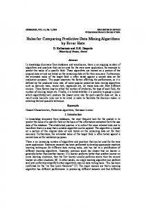
Fig. 1. Soil map of Italy (1:5,000,000) (Costantini et al., 2013).

The software packages used were ACCESS 2007 (Microsoft®) for queries of the soil geodatabase, ARCGIS 10.0 (Esri®) for spatial queries and cartographic restitutions and STATISTICA 10 (StatSoft®) for statistical analyses. Table 1 Hierarchy of Italian soilscapes and geodatabases. Soilscape level

Reference scale

Reference polygon size

Soil regions Soil subregions Soil systems Soil subsystems Soil units Soil element

1:5,000,000 1:1,000,000 1:500,000 1:250,000 1:50,000 1:10,000–25,000

105–106 104–105 103–105 102–105 101–102 10−1–101

ha ha ha ha ha ha

2.2. Methods 2.2.1. Selection of test areas To facilitate the comparison, the different approaches were tested in a subset of Italian soil regions. We selected 5 of the 10 soil regions in order to cover half of the Italian surface area. The regions were selected so that they would represent different profile densities. 2.2.2. Data preparation All auxiliary information was assigned to grid nodes of a 1 × 1-km spaced grid and attributed to 22,015 available classified soil profiles. In every SR the original dataset was divided into two parts: a training dataset for model building and a test dataset for both model selection and comparison of the final outputs. The size of the test dataset was

240

R. Lorenzetti et al. / Geoderma 237–238 (2015) 237–245

Table 2 Properties of the auxiliary variables. Variable

Original format

Type

Original reference scale or definition

Lithology Land-use DEM Slope Soil aridity index Carbon stock Soil inorganic carbon content Clay Sand Geography of soil systems

Polygons Grid Grid Grid Grid Grid Grid Polygons Polygons Polygons

Categorical Categorical Numerical Numerical Numerical Numerical Numerical Numerical Numerical Categorical

1:500,000 100 m 100 m 100 m 1 km 1 km 1 km 1:500,000 1:500,000 1:500,000

10% of total profiles in the five SRs. Since we needed to manage the clustering of the soil sites, the profiles of the validation dataset were chosen randomly and separately for each RSG. In this way, the dataset was able to represent every WRB class proportionally to its presence in the original dataset. The test datasets maintained the proportion of both the occurrence of the classes and their geographical distribution. Consequently, the number of test sites was higher for the more frequent RSGs and in the more densely sampled areas. The test dataset was kept out before the data processing. 2.2.3. Statistical methods Data mining techniques were tested as a possible alternative to the determinist approach in estimating the frequency of WRB classes in the legend of the 1:5,000,000 soil region map. Fig. 2 depicts the flowcharts of the deterministic and data mining methods. 2.2.3.1. Data mining. The ability of different techniques to predict RSGs through auxiliary variables was compared, namely neural networks, random forests, boosted tree, classification and regression tree, and supported vector machine. A neural network is a computational model emulating a biological neural system (Haykin, 1994; Singh and Chauhan, 2009). It is usually used to model complex relationships among variables or to find patterns in data. A random forest (Breiman, 2001) consists of an arbitrary number of simple trees, which are used to vote for the most popular class. Each tree is grown with a randomized subset of predictor values of the original dataset. A large number of trees (500 to 2000) is grown, hence a “forest”. The number of predictors used to find the best split at each node is a randomly chosen subset of the total number of predictors (Prasad et al., 2006). The boosted tree is a method to improve model accuracy based on the idea that finding a single, highly accurate prediction rule is harder than finding (and then averaging) many rough rules of thumb (Schapire, 2003). Unlike random forest, which merges results from multiple trees, boosting uses models sequentially. A random sample of data is selected at each step of the boosting process. The trees constructed during the process are summed, and each observation is classified according to the most common classification among the trees (Friedman, 1999, 2002). A classification and regression tree is a classification tree analysis developed by Breiman et al. (1984). The purpose is to determine, by means of tree-building algorithms, a set of if-then logical conditions that permit accurate prediction or classification of cases. Decision trees are constructed in a top-down recursive manner starting with a training set of records and their associated class labels. The training dataset is recursively partitioned into smaller subsets as the tree is being built (Han and Kamber, 2000). A supported vector machine (SVM) is a type of universal learning machine (Cortes and Vapnik, 1995; Vapnik, 2000). It is a learning algorithm used for pattern recognition and classification and was originally designed to solve binary classification problems (Hahn and Gloaguen, 2008). A SVM is based on the concept of “decision plane”, i.e. a plane able to separate a set of objects having different class memberships. The idea behind SVM is to map input data into a

Fig. 2. General data processing flows. A: deterministic approach; B: data mining approach.

higher dimensional space where a hyperplane can be constructed to separate classes (Hahn and Gloaguen, 2008). SVM moves data in the space through kernel mathematical functions. Objects are rearranged to produce a feature space where data of different class memberships are linearly separable. Statistica data miner recipes (SDMR) is a user interface for predictive data mining introduced by StatSoft. It consists of an automatic model builder and wizard-like data miner recipes to compare results of several methods applied to the same dataset. SDMR involved the following main steps. - Data for analysis: the original dataset was divided into training and test datasets as mentioned before. - Model building: the selected techniques, supported vector machine, neural network, random forest, boosted tree, and classification and regression tree, were applied to the training dataset for model building.

R. Lorenzetti et al. / Geoderma 237–238 (2015) 237–245

241

Table 3 Attributes of the Italian soil regions (the selected soil regions are in italics and bold type). Soil region (code)

A

B

C

D

E

F

G

H

I

L

Mean

Median

km2 Profile density (sites km−2) RSGs (n) Total profiles (n)

50,045 0.02 17 1001

35,177 0.07 25 2462

10,820 0.06 16 641

47,851 0.09 22 4171

30,001 0.07 22 2152

13,066 0.13 12 1699

47,772 0.08 21 3822

15,883 0.05 20 798

17,527 0.21 18 3743

26,977 0.24 25 6453

29,512 0.10 19.8 2637

28,489 0.08 20.5 2307

- Evaluation: models were applied to both the training and test datasets and the software reported the rate of cases incorrectly predicted by the five different techniques. - Deployment: the best model was applied to values of the grid dataset for the prediction of RSGs. Alphanumeric output was converted into a grid by ArcGIS to produce SR maps and used to calculate the five most frequent RSGs in each SR.

2.2.3.2. Bayesian validation. The Bayesian methodology is able to assess both positive and negative predictivities and this ability can be particularly useful when it is applied to estimate the uncertainty of the reported soil classes in a map legend. The Bayesian approach is similar to a natural learning process in which knowledge is improved by combining past and present experiences. We can say that it is a mathematical way to take into account expert knowledge in a statistical analysis. The central idea of the Bayesian approach is to combine likelihood (data) with prior knowledge (prior probability) to produce a revised probability (posterior probability) (Lesaffre and Lawson, 2012). In Bayes' predictive values, the pre-test odds of a hypothesis being true multiplied by the weight of new evidence (likelihood) generates post-test odds of the hypothesis being true (Gill et al., 2005). The Bayesian approach yields a conditional probability reflecting the context in which the test is applied (Gill et al., 2005). The positive predictive value of a model expresses the probability that an event occurs when the model estimates it to occur; it is a

Table 4 Soil distribution among the RSGs in the selected soil regions. WRB AB AC AL AN AR AT CH CL CM CR FL GL GY HS KS LP LV LX PH PL PT PZ RG SC SN ST UM VR Total

D 22 2 127 77 3 1 183 1312 357 100

E

H

I

L

4 1 17 21 27

1 2 15 143 10

1 48

1 1 25 23 149

15 150 899 1 46 6

4 32 141

93 320 466

217 1023 845

20 2

61

490 61

5 18 11 9 1424 102 10 4

52 97 191 4 85

194

1 1 346

3 126 16 76 4177

3 75 110 2152

7 115 50 101

47 161 1469 8 477

101 2

336 1

2 26 24 798

21 4 225 3743

11 315 155 1417 4 519 32 1 409 5 4 71 18 657 6453

measure of the confidence with which the presence of a phenomenon is predicted. On the other hand, the negative predictive value of a model expresses the probability that an event does not occur when the model estimates it to not occur; it is a measure of the confidence with which the absence of a phenomenon is predicted. In our case, the Bayesian methodology was applied to the test dataset to compare predictivity of the SVM and DA methods. The positive predictive value represented the probability that the observed RSG of the test dataset was the same as the predicted one. The negative predictive value represented the probability that the profiles not having the target RSG were predicted to belong to other RSGs. They were calculated as follows (Lesaffre and Lawson, 2012): predþ ¼

Se  prev
 Se  prev þ 1−Sp  ð1−prevÞ

pred− ¼

Sp  ð1−prevÞ Sp  ð1−prevÞ þ ð1−SeÞ  prev

where: pred+ pred− Se

is the positive predictive value. is the negative predictive value. is the sensitivity of the model, calculated as the ratio between the number of profiles correctly predicted in a specific RSG and the total number of observed profiles belonging to that RSG. is the specificity of the model, calculated as the ratio between Sp the number of evidences of absence of a specific RSG correctly predicted by the model and the total number of evidences of absence of that RSG. prev (prevalence) is the ratio between the number of evidences of presence of a RSG and the total number of profiles in the SR. The positive and negative predictive values were calculated separately for all the RSGs of each studied SR. Lists of the five most frequent RSGs resulting from the two methods were compared, as well as the positive and negative predictive values. In addition, a spatial Bayesian validation of the RSG prediction obtained with the methods was carried out on an exemplary soil region. The two maps showed the distribution pattern of the RSGs obtained with the methods at a more detailed scale, namely that of the soil systems. The similarity between the lists given by the two methods was estimated through Spearman's rank correlation coefficient (ρ). The Spearman test provides a coefficient of correlation between two variables based on ranks of measurements and not actual values. Spearman's rank correlation coefficient can be considered a Pearson correlation coefficient between ranked variables and ρ is computed as follows:

X

ðx −xÞðyi −yÞ i i ρ ¼ qffiffiffiffiffiffiffiffiffiffiffiffiffiffiffiffiffiffiffiffiffiffiffiffiffiffiffiffiffiffiffiffiffiffiffiffiffiffiffiffiffiffiffiffiffiffiffiffiffiffi X X 2 2 ðx −xÞ ðy −yÞ i i i i

242

R. Lorenzetti et al. / Geoderma 237–238 (2015) 237–245

Fig. 3. Map of the five studied soil regions with the predicted RSGs in order of occurrence.

where xi and yi are ranks of the raw scores X, Y of the observation i. The formula has a simplified version when there are no tied ranks: X 2 6 di  ρ ¼ 1−  2 n n −1

3. Results

where d is the difference between the ranks of each observation i of the two variables and n is the number of pairs. Table 5 Competitive evaluation of the data mining models (SVM: supported vector machine; NN: neural network; RF: random forest; BT: boosted tree; C&RT: classification and regression tree).

SVM NN RF BT C&RT

In our ρ computation, we compared the lists of the first five RSGs. In the SRs where the first five RSGs were not the same, the absent RSGs were added to the lists.

SR D Error (%)

SR E Error (%)

SR H Error (%)

SR I Error (%)

SR L Error (%)

Train

Test

Train

Test

Train

Test

Train

Test

Train

Test

32.4 46.0 92.0 48.8 92.0

67.9 66.0 98.1 73.5 98.1

16.8 45.6 95.9 49.9 97.5

60.0 87.3 98.2 65.5 100.0

22.6 71.4 97.1 57.4 97.4

72.0 96.0 100.0 72.0 100.0

25.6 48.3 98.3 43.9 98.3

51.8 98.2 98.2 53.7 98.2

31.7 51.0 96.9 59.6 96.9

76.6 56.7 99.3 78.7 99.3

3.1. Studied soil regions The selected soil regions, covering about half of the total surface area of the country, were the following (Table 3): “Soils of the Po plain and associated hills” (D; 4,785,090 ha); “Soils of the central and southern Table 6 Spearman rank order correlations (DA vs SVM). SR

No. ranks

Spearman R

p-Value

D E H I L Mean

6 8 6 6 7

0.54 0.68 0.37 0.37 0.38 0.47

0.266 0.066 0.468 0.468 0.398 0.330

R. Lorenzetti et al. / Geoderma 237–238 (2015) 237–245 Table 7 Mean values of the positive and negative predictive values. SR

D E H I L Mean

No. tests

411 168 93 370 1706

SVM

DA

pred+

pred−

pred+

pred−

0.381 0.592 0.348 0.246 0.404 0.442

0.946 0.994 0.877 0.934 0.949 0.941

0.213 0.222 0.202 0.240 0.225 0.220

0.948 0.895 0.890 0.965 0.937 0.927

243

the two approaches in each SR. The RSGs are listed in order of occurrence. The colors in the legend identify the soil regions in the map. Following the WRB rules for creating map legends, SR D had two codominants (40.3% and 32.8%) and one associated (15.4%) RSG; SR E had one dominant (65.6%) and one associated (16.2%) RSG only; SR H had one dominant (51.7%) and four associated (11.1%; 10.6%; 10.2% and 7.2%) RSGs; SR I had one codominant (31.9%) and five associated (16.7%; 15.2%; 11.8%; 9.0% and 7.6%) RSGs; and SR L had two codominants (31.0% and 28.8%) and two associated (12.9% and 8.3%) RSGs. 4. Discussion

Apennines” (E; 3,000,072 ha); “Soils of hills of central and southern Italy formed on volcanic deposits and limestone” (H; 1,588,328 ha); “Soils of hills and marine terraces of southern Italy, formed on calcareous sediments” (I; 1,752,656 ha); and “Soils of plains and low hills of central and southern Italy” (L; 2,697,745 ha). The amount of soil profiles of each RSG in the SRs is reported in Table 4. The profile density ranged from low in soil region H (0.05 sites km−2, lower than the first quartile) to medium in soil regions D and E (respectively 0.09 and 0.08 sites km−2, near the median density) to high in I and L (respectively 0.22 and 0.24 sites km−2). The five most frequent RSGs in the SRs (according to the DA) are reported in Fig. 3 in their order of estimated area coverage.

4.1. Ranking the legend taxa The two approaches differentiated the order of RSG classes (Fig. 3). In fact, according to the Spearman correlation index, the SVM and DA legends were not correlated (Table 6), which means that the two approaches produced significantly different outcomes. The RSGs named in the lists were almost always identical, but the differences increased with decreasing occurrence. In fact, the most widespread RSG was always the same, while the second position was the same only in L and E, and the other positions had never the same RSGs. 4.2. Bayesian validation

3.2. Data mining approach Comparison of the different data mining techniques indicated the SVM model as the best method to predict RSGs (Table 5). In the test dataset, the SVM model produced the minimum error rate in three of five SRs, while it always gave the minimum error rate in the training dataset. Therefore, SVM was chosen for comparison with the deterministic approach. The five most frequent RSGs resulting from the predicting models are reported in Fig. 3. The figure compares the legends obtained with

4.2.1. Bayesian validation of the RSG frequencies in the legend of the soil region map The Bayesian validation showed that both methods had a much higher negative than positive prediction ability. This was a consequence of the much larger number of evidences of absence than presence of a specific RSG. In fact, a strong point of the Bayesian approach in the estimation of the prediction power is that a given corrected prediction (Se, Sp) may generate different predictive values (pred +; prev−), since prev+ (−) takes also into account the prevalence (prev) of the

Fig. 4. Vectorial map from DA of soil region D, with the distribution of the test profiles. AB — Albeluvisols; AL — Alisols; AR — Arenosols; CL — Calcisols; CM — Cambisols; FL — Fluvisols; GL — Gleysols; HS — Histosols; LP — Leptosols; LV — Luvisols; PH — Pheozems; RG — Regosols; ST — Stagnosols; UM — Umbrisols; VR — Vertisols.

244

R. Lorenzetti et al. / Geoderma 237–238 (2015) 237–245

Fig. 5. Grid map from SVM of soil region D, with the distribution of the test profiles.

target class in the test dataset and, in our case, the amount of observed absences of a RSG in the test dataset was always much higher than the observed presences. In addition, it is noticeable that the negative predictive values resulted comparable, whereas the mean positive predictive values well differentiated the methods. SVM showed higher pred+ than DA (Table 7). The highest mean positive pred + was obtained with SVM in the Apennine soil region (E), although the outcomes were very variable both among and within the SRs. It must be also underlined that SR E was also the most characterized one, according to WRB rules for naming soil maps (one dominant and one associated RSG only). On the contrary, SR I showed the lowest pred+ and also the larger presence of associated RSGs, because of the lack of dominant soils.

the most frequent soil classes, but they have very different predictability. Actually, it is well known that Luvisols and Vertisols are often strongly spatially correlated with the factor of pedogenesis, differently from Cambisols, which can be found in contrasting environments (Wilding et al., 1983). On the other hand, well predictable Vertisols have much fewer cases. This result confirms a stated strength of SVM, that it is able to provide good results even with a small number of training data points (Foody and Mathur, 2006; Kovačević, 2010). The low predictability of some RSGs instead could be attributed to the fact that the distribution of these soil taxa was not well constrained by the used covariates, while more detailed relationships, not included in the SVM model, played a major role. The scale of the lithological

4.2.2. Geographical pattern and predictability of RSGs Soil region D was chosen as an example to show the geographical pattern of RSGs within a soil region, because of its single polygon shape. As highlighted in Figs. 4 and 5, the spatial distribution of RSGs at the soil system scale, obtained with the two methodologies, was rather different, despite the comparable mean positive predictive values (Table 7). Although the aim of the work was not to detail the soil region map, but to improve the reliability of the legend, it is noteworthy that the polygons in the SVM map substantially followed the forms of the landscape and the delineations of soil systems. In fact, SVM did not lose the geographical relationship with the factors of pedogenesis, thanks to the strong link between environmental predictors and estimation. As regards the ability to predict a specific RSG, SVM showed perfect positive predictivity for five RSGs, namely Alisols, Gleysols, Vertisols, and Leptosols, while DA showed perfect positive predictivity only for Vertisols (Table 8). Luvisols, the most numerous taxon, was always rather well predicted, but Regosols, Stagnosols, Phaeozems, Albeluvisols, Histosols, Umbrisols, and Kastanozems were not or very little predictable by both methods. The positive predictability of RSGs with SVM cannot be simply due to the abundance of the training dataset. In fact, Luvisols and Cambisols are

Table 8 Bayesian positive (pred+) and negative (pred −) predictive values estimated in soil region D. Also reported are the abundance of soils in the test dataset (N test), the sensitivity (Se) and the specificity (Sp). DA

SVM

RGS

No. tests

Se

pred+

LV CM FL RG CL AL ST GL PH VR AR AB HS UM LP KS

141 131 36 19 18 13 13 10 10 8 7 2 2 2 1 1

0.936 0.506 0.687 0.373 0.333 0.140 0.526 0.073 0.722 0.141 0.000 0.000 Not available 0.300 0.035 0.000 0.000 0.625 1.000 0.125 0.077 Not available Not available Not available Not available Not available

Sp

pred−

Se

pred+

Sp

pred−

0.511 0.449 0.799 0.671 0.796 1.000

0.938 0.750 0.925 0.966 0.984 0.968

0.790 1.000 1.000 0.970

0.978 0.975 0.993 0.982

0.461 0.641 0.976 0.000 0.722 0.077 0.000 0.100 0.000 0.125 0.125 0.000 0.000 0.000 1.000 0.000

0.596 0.380 0.308 0.000 0.260 1.000 0.000 1.000 0.000 1.000 0.167 0.000 0.000 0.000 1.000 1.000

0.833 0.500 0.308 1.000 0.904 1.000 1.000 1.000 0.983 1.000 0.987 1.000 1.000 1.000 1.000 1.000

0.743 0.745 0.918 0.953 0.986 0.970 0.970 0.978 0.983 0.983 0.982 0.995 0.995 0.995 1000 0.998

R. Lorenzetti et al. / Geoderma 237–238 (2015) 237–245

map, for instance, could not have been adequate to reflect the variability of alluvial sediments. 5. Conclusions The results of this study indicate that the order of abundance of predicted RSGs in the legend of the soil region map differed significantly according to the inference model used, and the specific SR and RSG. The Bayesian validation demonstrated that positive predictive values were higher with the SVM. In particular, a more reliable prediction was obtained: i) in the SRs with a high occurrence of a dominant RSG and few associated soils; ii) for the RSGs that resulted more strongly correlated with the factors of pedogenesis. Nevertheless, negative predictions were similar and much higher than positive ones with both the DA and SVM methods. Actually, both legends were more reliable in showing the absence rather than the presence of the listed RSGs in each SR. Thus much soil variability remained uncontrolled, in spite of the improvements obtained with SVM. In conclusion, this research work suggests that the SVM method is better than the DA. A future challenge is to test the suitability of data mining to estimate soil class frequency in the legend of maps produced at more detailed scales or with other spatialization methodologies. References Adhikari, K., Minasny, B., Greve, M.B., Greve, M.H., 2013. Constructing a soil class map of Denmark based on the FAO legend using digital techniques. Geoderma http://dx. doi.org/10.1016/j.geoderma.2013.09.023. Barbetti, R., L'Abate, G., Priori, S., Costantini, E.A.C., 2012. Soil inorganic carbon stock of Italy. Proceedings of the 4th International Congress Eurosoil 2012. BGR, 2011. Soil Regions of the European Union and Adjacent Countries 1:5 000 000 (EUSR 5000) Version 2.0. , ([online] http://www.bgr.bund.de/EN/Themen/Boden/Projekte/ Informationsgrundlagen_abgeschlossen/EUSR5000/EUSR5000.html (verified 22.10. 2013)). Breiman, L., 2001. Random forests. Mach. Learn. 45, 5–32. Breiman, L., Friedman, J.H., Olshen, R.A., Stone, C.J., 1984. Classification and Regression Trees. Wadsworth & Brooks/Cole Advanced Books & Software, Monterey, CA. Carré, F., McBratney, A.B., Mayr, T., Montanarella, L., 2007. Digital soil assessments: beyond DSM. Geoderma 142 (1), 69–79. Cortes, C., Vapnik, V., 1995. Support-vector networks. Mach. Learn. 20 (3), 273–297. Costantini, E.A.C. (Ed.), 2007. Linee guida dei metodi di rilevamento e informatizzazione dei dati pedologici. SISS, Firenze, Italia, p. 296. Costantini, E.A.C., L'Abate, G., Barbetti, R., Fantappiè, M., Lorenzetti, R., Magini, S., 2012. “Carta dei suoli d'Italia. scala 1:1.000.000 (soil map of Italy scale 1:1.000.000”). Consiglio per la Ricerca e la sperimentazione in agricoltura — S.E.LC.A. Firenze. Italia. http://abp.entecra.it/soilmaps/ita/cartadeisuoli1.html Costantini, E.A.C., L'Abate, G., 2009. A soil aridity index to assess desertification risk for Italy. Land Degradation and Rehabilitation — Dryland Ecosystems. Catena, pp. 231–242. Costantini, E.A.C., Barbetti, R., Fantappiè, M., L'Abate, G., Lorenzetti, R., Magini, S., 2013. Pedodiversity. The Soils of Italy. Springer, Netherlands, pp. 105–178. De Jacher, A.L., 2012. Preparing CORINE land cover data for use. Optimization of Land Cover Data Using a Data Base and Topological GIS Platform. European Commission. Joint Research Center. Institute for Environmental and Sustainability 978-92-7922720-2, (EUR 25163 EN, (print)). Fantappiè, M., L'Abate, G., Costantini, E.A.C., 2010. Factors influencing soil organic carbon stock variations in Italy during the last three decades. Land Degradation and Desertification: Assessment. Mitigation and Remediation. Springer, pp. 435–465. Finke, P., Hartwich, R., Dudal, R., Ibanez, J., Jamagne, M., King, D., Montanarella, L., Yassoglu, N., 1998. Georeferenced Soil Database for Europe. JRC, EUR 18092, Ispra, Italy. Foody, G.M., Mathur, A., 2006. The use of small training sets containing mixed pixels for accurate hard image classification: training on mixed spectral responses for classification by a SVM. Remote Sens. Environ. 103 (2), 179–189.

245

Friedman, J.H., 1999. Greedy function approximation: a gradient boosting machine. IMS 1999 Reitz Lecture. . Friedman, J.H., 2002. Stochastic gradient boosting. Comput. Stat. Data Anal. 38 (4), 367–378. Gill, C.J., Sabin, L., Schmid, C.H., 2005. Why clinicians are natural Bayesians. BMJ Br. Med. J. 330 (7499), 1080. Hahn, C., Gloaguen, R., 2008. Estimation of soil types by non linear analysis of remote sensing data. Nonlin. Processes Geophys. 15, pp. 115–126 (www.nonlin-processesgeophys.net/15/115/2008/). Han, J., Kamber, M., 2000. Data Mining: Concepts and Techniques. Morgan-Kaufman, New York. Haykin, S., 1994. Neural Networks: A Comprehensive Foundation. Hudson, B.D., 1992. The soil survey as paradigm-based science. Soil Sci. Soc. Am. J. 56, 836–841. Ibañez, J.J., Feoli, E., 2013. Global relationships of pedodiversity and biodiversity. Vadose Zone J. 12. Ibañez, J.J., De-Alba, S., Lobo, A., Zucarello, V., 1998. Pedodiversity and global soil patterns at coarse scales (with discussion). Catena 83, 171–214. IUSS Working Group WRB, 1998. World reference base for soil resources. World Soil Resources Reports 84. ISSS, FAO, ISRIC, Rome, p. 99. IUSS working group WRB, 2014. World reference base for soil resouces 2014. International Soil Classification SYSTEM for Naming Soils and Creating Legends for Soil Maps, Word Soil Resources Reports No. 106FAo, Rome. Jenny, H., 1941. Factors of soil formation. A System of Quantitative Pedology. McGraw-Hill, New York. Jenny, H., 1980. The Soil Resource: Origin and Behaviour. Springer-Verlag, New York. Kovačević, M., 2010. Soil type classification and estimation of soil properties using support vector machines. Geoderma 154, 340–347. Kros, J., Pebesma, E.J., Reinds, G.J., Finke, P.A., 1999. Uncertainty assessment in modelling soil acidification at the European scale: a case study. J. Environ. Qual. 28 (2), 366–377. Lagacherie, P., 2008. Digital soil mapping: a state of the art. Digital Soil Mapping With Limited Data. Springer, Netherlands, pp. 3–14. Lemercier, B., Lacoste, M., Loum, M., Walter, C., 2012. Extrapolation at regional scale of local soil knowledge using boosted classification trees: a two-step approach. Geoderma 171–172, 75–84. Lesaffre, E., Lawson, A.B., 2012. Bayesian Biostatistics. John Wiley & Sons, UK 978-0-47001823-1, pp. 16–17. McBratney, A.B., Mendonça Santos, M.D.L., Minasny, B., 2003. On digital soil mapping. Geoderma 117 (1), 3–52. Mendonça-Santos, M.L., Santos, H.G., Dart, R.O., Pares, J.G., 2008. Digital mapping of soil classes in Rio de Janeiro state. Brazil: data. Modelling and prediction. Digital Soil Mapping With Limited Data, pp. 381–396. MIPAF, 2000. Metodi di Analisi Chimica. Ministero Delle Politioche Agricole E Forestali. Franco Angeli Editore, Milano. Italia. Moonjun, R., Farshad, A., Shrestha, D.P., Vaiphasa, C., 2010. Artificial neural network and decision tree in predictive soil mapping of Hoi Num Rin sub-watershed. Thailand. Digital Soil Mapping. Springer, Netherlands, pp. 151–164. Oleg, A., Nikola, P., Sven, D.J., 2003. Spatial distribution of main forest soil groups in Croatia as a function of basic pedogenetic factors. Ecol. Model. 170, 363–371. Prasad, A.M., Iverson, L.R., Liaw, A., 2006. Newer classification and regression tree techniques: bagging and random forests for ecological prediction. Ecosystems 9, 181–199. http://dx.doi.org/10.1007/s10021-005-0054-1. Righini, G., Costantini, E.A.C., Sulli, L., 2001. La banca dati delle regioni pedologiche italiane. Boll. Soc. Ital. Sci. Suolo 50, 261–271. Schapire, R., 2003. The boosting approach to machine learning — an overview. In: Denison, D.D., Hansen, M.H., Holmes, C., Mallick, B., Yu, B. (Eds.), MSRI Workshop on Nonlinear Estimation and Classification. 2002. Springer, New York. Servizio geologico d'Italia, 1978. Carta geologica d'Italia in scala 1:500.000. Singh, Y., Chauhan, A.S., 2009. Neural networks in data mining. J. Theor. Appl. Inf. Technol. 5 (1), 37–42. Soil Survey Division Staff, 1993. Soil Survey Manual. Agricultural Handbook N 18. USDA Natural Resources Conservation Service, Washington D.C., USA, p. 438. Soil Survey Staff, 1999. Soil taxonomy: a basic system of soil classification for making and interpreting soil surveys, Natural Resources Conservation Service2nd edition. U.S. Department of Agriculture Handbook 436. Vapnik, V.N., 2000. The Nature of Statistical Learning Theory (Statistics for Engineering and Information Science), Second edn. Springer Verlag, p. 314. Wilding, Larry P., Smeck, Neil E., Hall, G.F., Wilding, Larry P., Smeck, Neil E., Hall, G.F., 1983. Pedogenesis and soil taxonomy: the soil orders. The Soil Orders vol. 11. Elsevier. Zhu, A.X., Hodson, B., Burt, J., Lubich, K., Simonson, D., 2001. Soil Mapping using GIS, expert Knowledge, and fuzzy logic. Soil Sci. Soc. of Am. J. 65 (5), 1463–1472.