Comparing Mixture Estimates by Parametric Bootstrapping Likelihood Ratios Joel H. REYNOLDS and William D. TEMPLIN Wildlife managers and researchers often need to estimate the relative contributions of distinct populations in a mixture of organisms. Increasingly, there is interest in comparing these mixture contributions across space or time. Comparisons usually just check for overlap in the interval estimates for each population contribution from each mixture. This method in ates Type I error rates, has limited power due to its focus on marginal comparisons, and employs a fundamentally inappropriate measure of mixture difference. Given the dif culty of de ning an appropriate measure of mixture difference, a powerful alternative is to compare mixtures using a likelihood ratio test. In applications where the standard asymptotic theory does not hold, the null reference distribution can be obtained through parametric bootstrapping. In addition to testing simple hypotheses, a likelihood ratio framework encourages modeling the change in mixture contributions as a function of covariates. The method is demonstrated with an analysis of potential sampling bias in the estimation of population contributions to the commercial sockeye salmon (Oncorhynchus nerka) shery in Upper Cook Inlet, Alaska. Key Words: Compositional data; Compositional difference; Discrete mixture analysis; Genetic stock identi cation; Mixed stock analysis; Mixture homogeneity.
1. INTRODUCTION Mixed stock analysis (MSA) estimates the relative contributionsof distinct populations in a mixture of organisms. MSA is an important tool in sheries management and research (Begg, Friedland, and Pearce 1999; Shaklee, Beacham, Seeb, and White 1999), marine mammal research (Pella and Masuda 2001), and wildlife management and conservation (Pearce et al. 2000). The underlying approach has been applied to problems ranging from estimating the percentage of genes from source or parental populations(Planes and Doherty 1997) to eld investigations of owl diets (Do and McLachlan 1984). Although methods for Joel H. Reynolds is Biometrician, U. S. Fish and Wildlife Service, Division of Natural Resources, 1011 E. Tudor Road, MS 221, Anchorage, AK 99503 (E-mail: Joel
[email protected]). William D. Templin is Fisheries Geneticist, Gene Conservation Laboratory of the Commericial Fisheries Division, Alaska Department of Fish and Game (E-mail: Bill Templin@ shgame.state.ak.us). ® c 2004 American Statistical Association and the International Biometric Society Journal of Agricultural, Biological, and Environmental Statistics, Volume 9, Number 1, Pages 57–74 DOI: 10.1198/1085711043145 57
58
J. H. REYNOLDS AND W. D. TEMPLIN
MSA estimation have appeared in the sheries literature for many years (e.g., Cassie 1954; Grant, Milner, Krasnowski, and Utter 1980; Pella and Milner 1987), and much longer in the statistics literature (see the extensive surveys in Blischke 1963; Redner and Walker 1984; Titterington, Smith, and Makov 1985; McLachlan and Peel 2000), new applications continually require methodological extensions. There is growing interest in mixture homogeneity in space or time. Researchers assess differences in mixture estimates from independent samples by looking across the samples for overlap of the con dence intervals for a given population’s contribution (e.g., Wilmot, Kondzela, Guthrie, and Masuda 1998; McParland, Ferguson, and Liskauskas 1999; Seeb and Crane 1999; Shaklee et al. 1999; Ruzzante, Taggart, Lang, and Cook 2000). This approach suffers from both in ated Type I error rates due to multiple testing and in ated Type II error rates due to focusing on marginal summary statistics. The approach employs a fundamentally inappropriate measure of mixture difference that ignores the dependence among contribution estimates arising from their constrained sum (see Section 5). MSA commonly uses maximum likelihood estimation; we extend this framework to a conditional likelihood ratio test of mixture homogeneity across independent samples, similar in avor to McLachlan’s (1987) approach to testing the number of mixture components. Asymptotic theory, Monte Carlo simulation, or parametric bootstrapping provide approximate P values. In addition to testing simple hypotheses, a likelihood ratio framework encourages explicit modeling of mixtures as functions of covariates. The method is implemented in the latest release of the freeware Statistical Package for Analyzing Mixtures [SPAM; version 3.6 (Reynolds 2001) available online at http: //www.cf.adfg.state.ak.us/geninfo/research/genetics/software/spampage.php]. Section 2 presents a motivating application from the sockeye salmon (Oncorhynchus nerka) commercial shery in Upper Cook Inlet, Alaska, then Section 3 introduces the basic nite mixture model, derives the likelihoodratio test of M -sample mixture homogeneity,and presents three approaches to approximating the null reference distribution. Section 4 shows how parametric bootstrapping is used to test mixture homogeneity for the sockeye salmon data. Section 5 compares the performance of the likelihood ratio method and the con dence interval method both for the current application and in general. Marginal measures of “mixture difference” appropriate to compositionaldata are brie y discussed. The Appendix extends the nite mixture model to two-stage sampling.
2. APPLICATION: COMPARING SALMON HARVEST MIXTURES The sockeye salmon shery in Upper Cook Inlet, Alaska (Figure 1) is a major component of the local economy. Over the last ten years, the total annual value of commercial sheries harvests in the region ranged from US $8.8 to $111.1 million, with sockeye salmon comprising 80%–97% of the annual value (Ruesch and Fox 1999). The shing eet is very ef cient; the approximately 600 drift gillnet vessels can harvest as much as 70% of the available sh in a single 12-hour opening (Seeb et al. 2000).
COMPARING MIXTURE ESTIMATES
59
Most sockeye salmon home with precision, returning from the ocean to their natal habitats to spawn and then die (Burgner 1991). Adults may spawn in many diverse environments (i.e., rivers, sloughs, lake shores), but survival of their offspring generally depends on the offspring successfully emigrating shortly after emergence to rear in a lake. This reliance on rearing lakes is characteristic of the majority of the species, and contrasts with the other Paci c salmonids (Burgner 1991). Over time, the low rates of straying (spawning in a
Figure 1. Upper Cook Inlet, Alaska. Numbers locate each baseline population listed in Table 1 (from Seeb et al. 2000). Commercial harvests occurred in the Central District.
J. H. REYNOLDS AND W. D. TEMPLIN
60
Table 1. Baseline Populations and Associated Reporting Regions for the Mixture Analysis of Commercially Harvested Sockeye Salmon in Upper Cook Inlet, Alaska from Seeb et al. (2000) Region West Cook Inlet Susitna/Yenta
Knik Northeast Cook Inlet Kenai Kasilof
Population 1–Chilligan R., 2–Crescent Lk., 3–Wolverine Ck., 4–McArthur R., 5– Packers Lk., 6–Coal Ck. 7–Yentna R., 8–Shell Lk., 9–Hewitt/Whiskey Lks., 10–Trinity/Movie Lks., 11–Judd Lk., 12–Chelatna Lk., 13–Byers Lk., 14–Susitna R., 15–Mama & Papa Bear Lks., 16–Larson Lk., 17–Talkeetna R., 18– Stephan Lk., 19–Birch Ck., 20–Red Shirt Lk. 21–Nancy Lk., 22–Cottonwood Lk., 23–Fish Ck., 24–Jim Ck., 25– Sixmile Ck. 26–Daniels Lk., 27–Bishop Ck., 28–Swanson R. 29–Skilak Lk. Outlet, 30–Hidden Ck., 31–Between Kenai and Skilak Lk., 32–Upper Russian R., 33–Tern Lk., 34–Quartz Ck., 35–Moose Ck., 36–Johnson Ck., 37–Railroad Ck., 38–Ptarmigan Ck. 39–Nikolai Ck., 40–Tustumena Lk., 41–Bear Ck., 42–Moose Ck., 43– Glacier Ck., 44–Seepage Ck.
NOTE: Numbers refer to labels in Figure 1. Ck.–Creek, Lk.–Lake, R.–River.
location other than the natal habitat) and the demands of different spawning environments can lead to signi cant genetic, morphometric, and behavioral differences between sockeye populations within a relatively small geographic area (e.g., Woody, Olsen, Reynolds, and Bentzen 2000). Maintaining genetic diversity and future productivity in the face of more immediate demands for economic returns by highly ef cient shers requires that shery managers accurately identify the harvest contributions of the major Upper Cook Inlet sockeye salmon stocks. Sustainable management will be very dif cult, if not unachievable, otherwise. There are 44 genetically distinct populations, or stocks, within the major sockeye salmon-producing areas of Upper Cook Inlet (Seeb et al. 2000). Overharvesting any of the stocks reduces both the region’s genetic diversity, through loss of unique combinations of genetic characters, and the shery’s economic value, as lost stocks will not contribute to future harvests.
2.1
THE PROBLEM
The mixture of interest is the sockeye harvest in the Central District shery during a 12-hour opening (Figure 1). Each boat delivers its catch to 1 of 11 processors. Traditionally, the harvest was sampled only at the largest processor, Wards Cove (Seeb et al. 2000). To ascertain whether this procedure produces biased mixture estimates, replicate samples from a second processor, Salamatof Seafoods, Inc., were collected on four openings during the 1997 and 1998 seasons. We wish to test the equality of the mixture estimates from the two processors.
2.2
THE DATA
Previous mixed stock analyses on Upper Cook Inlet sockeye have used scale patterns (Marshall et al. 1987), parasites (Waltemeyer, Tarbox, and Brannian 1993), and genetic
COMPARING MIXTURE ESTIMATES
61
markers (Grant et al. 1980; Seeb et al. 2000). Of these characteristics, genetic markers provided the most accurate and precise mixture estimates (Seeb et al. 2000). Samples of spawning salmon were collected from each of the 44 baseline populations (Figure 1, Table 1) (Seeb et al. 2000), with a target sample size of 100 individuals per population (Allendorf and Phelps 1981; Waples 1990). Allozyme electrophoresis was used to detect each individual’s genotype at 27 discriminating unlinked neutral loci [Seeb et al. (2000) detailed the tissue collection, loci, laboratory analyses, population genetic analyses, and results]. Geography (Figure 1) and genetic diversity (Figure 2), followed by extensive simulation analyses, were used to de ne six regions, or population aggregates, that were reliably identi ed in mixture estimation (Seeb et al. 2000). A region had to demonstrate a contribution estimate of ¶ 90%, averaged over 500 bootstrap resamples, from simulated
Figure 2. Neighbor-joining tree (Saitou and Nei 1987) of Cavalli-Sforza and Edwards chord length genetic distances (Cavalli-Sforza and Edwards 1967) between Upper Cook Inlet sockeye salmon populations (Table 1, Figure 1). Genetic distances are calculated from 27 unlinked allozyme electrophoresis loci (data in Seeb et al. 2000). Regional membership of each population is indicated in the right-hand column.
62
J. H. REYNOLDS AND W. D. TEMPLIN
mixture samples of 400 genotypes, where each mixture sample was drawn uniformly from the populations within the region of interest, and each genotype was parametrically bootstrapped from its population of origin’s allele frequency estimates. Six regions were thus identi ed (Figure 1, Figure 2): Kenai, Kasilof, West Cook Inlet, Susitna/Yentna, Knik, and Northeast Cook Inlet. Most sockeye salmon come from the rst four regions (Tobias and Tarbox 1999), all of which contain major river drainages (Figure 1). The mixture sample at each processor was obtained by two-stage sampling: boats were randomly sampled from the incoming sequence of deliveries, and a random sample of sockeye salmon were selected from each boat’s catch. Forty boats were sampled at Wards Cove at a rate of 10 sh per boat, for a target sample size of 400 sh per period. Salamatof Seafoods Inc., the smaller processor, serves a eet of 20–30 boats. In 1997, 10 to 15 sh were sampled per boat depending on the number of boats returning, for a target sample size of 400 sh per period. In 1998, the goal was revised to 10 sh per boat for a target of 200 sh per period. Allozyme electrophoresis was used to detect each individual’s genotype at the 27 loci previously used to characterize the baseline populations [Seeb et al. (2000) detailed the genetic tissue collection, laboratory analysis, and results].
3. METHODS 3.1
THE FINITE MIXTURE MODEL
A friend goes into a candy store. Two large jars contain both strawberry and licorice candies, but in different proportions. She randomly grabs some candy from each well-mixed jar (the baseline populations), places it a single bag (the mixture), pays for it, walks out, and hands it to you. She tells you the original proportions in each jar, then says you may have some candy if you can tell her what portion of the mixture came from each jar. This is a nite mixture problem (only two jars contributed) with a discrete characteristic ( avor) and known source population characteristics ( avor proportions in each jar). Mixture identi ability requires that the probability density functions of the characteristics (e.g., avors) are linearly independent across the set of populations (e.g., jars) [Teicher (1963) and Redner and Walker (1984) provided a survey of general identi ability results; Lindsay (1995) provided a thorough discussion for mixtures of discrete characteristics]. Characteristics commonly used in sheries include parasite assemblages (Moles and Jensen 2000; Urawa, Nagasawa, Margolis, and Moles 1998), scale patterns (Marshall et al. 1987), morphometrics and meristics (Fournier, Beacham, Ridell, and Busack 1984), arti cial tags such as thermal marks, coded wire tags, or n clips (Ihssen et al. 1981) and, increasingly, genetic markers (Seeb and Crane 1999; Ruzzante et al. 2000). The following presentation assumes a discrete characteristic, though this assumption is not essential. Let n items be randomly sampled from a mixture of J populations. Let the jth population contribute an unknown proportion ³ j ¶ 0 to the mixture, §³ j = 1; µ = (³ 1 ; : : : ; ³ J ). e If the characteristic measured on the ith sample observation is denoted by xi , then the probability of observing the sample X = fx1 ; x2 ; : : : ; xn g is e
COMPARING MIXTURE ESTIMATES
Pr(Xjµ; ¼ ) = e e e
n Y
i= 1
µ
Pr xi jµ ; ¼ e e
¶
=
8 n