Main result. Application to multiple testing. Comparison of methods. Conclusion g(x) = af (x)+(1âa)Ï(x). Idea Build a kernel nonparametric estimate of f using the.
Introduction General approach Main result Application to multiple testing Comparison of methods Conclusion
A semi-parametric approach for mixture models, application to local False Discovery Rate estimation Jean-Jacques Daudin, Ag r oPar i sTech/INRA, joint work with S. Robin, A. Bar-Hen, L. Pierre (Univ. Paris X)
Jean-Jacques Daudin, Ag r oPar i sTech/INRA, joint work with S. Robin, A.ABar-Hen, semi-parametric L. Pierre approach (Univ. Paris forX)mixture models, application to local F
Introduction General approach Main result Application to multiple testing Comparison of methods Conclusion
Mixture model
two-populations g (x) = a f (x) + (1 − a)φ(x) probability density function φ is known probability a is unknown probability density function f is unknown.
Jean-Jacques Daudin, Ag r oPar i sTech/INRA, joint work with S. Robin, A.ABar-Hen, semi-parametric L. Pierre approach (Univ. Paris forX)mixture models, application to local F
Introduction General approach Main result Application to multiple testing Comparison of methods Conclusion
Applications Contamination problems, distribution φ is known, contamination distribution f is unknown, proportion a of contamination is unknown.
Data set relating to speed of light measurements made by Simon Newcomb (in Gelman et al in Bayesian Data Analysis (2004))
Multiple testing problems p-values under H0 are uniformly distributed on [0, 1], φ is the uniform distribution, distribution of the p-values associated to H1 is unknown, proportion a of observations under H1 is unknown.
Jean-Jacques Daudin, Ag r oPar i sTech/INRA, joint work with S. Robin, A.ABar-Hen, semi-parametric L. Pierre approach (Univ. Paris forX)mixture models, application to local F
Introduction General approach Main result Application to multiple testing Comparison of methods Conclusion
g (x) = a f (x) + (1 − a)φ(x) Idea Build a kernel nonparametric estimate of f using the information we have on φ Issue It is easy to build a kernel density of the overall distribution g , but that is not what we want to do we want to build a kernel estimate of f , so we need to know which observations are generated under f . this information is not available... Solution Estimate the probability for each observation of being generated under f (or under φ).
Jean-Jacques Daudin, Ag r oPar i sTech/INRA, joint work with S. Robin, A.ABar-Hen, semi-parametric L. Pierre approach (Univ. Paris forX)mixture models, application to local F
Introduction General approach Main result Application to multiple testing Comparison of methods Conclusion
Basic relation 1
Consider an observation x Assume that f and a are known, The probability τ(x) that this observation has been generated under f is τ(x) =
a f (x) a f (x) = ... g (x) a f (x) + (1 − a)φ(x)
But f and a are unknown, we just wanted to estimate them !
Jean-Jacques Daudin, Ag r oPar i sTech/INRA, joint work with S. Robin, A.ABar-Hen, semi-parametric L. Pierre approach (Univ. Paris forX)mixture models, application to local F
Introduction General approach Main result Application to multiple testing Comparison of methods Conclusion
Basic relation 2 The standard kernel estimate of f is " #, X X fb(x) = Z i k i (x) Zi . i
i
where k is a kernel pdf k i (x) = k[(x − x i )/h]/h h is the bandwidth of the kernel Z i is one if the data x i comes from f and 0 otherwise.
Jean-Jacques Daudin, Ag r oPar i sTech/INRA, joint work with S. Robin, A.ABar-Hen, semi-parametric L. Pierre approach (Univ. Paris forX)mixture models, application to local F
Introduction General approach Main result Application to multiple testing Comparison of methods Conclusion
Basic relation 2 " fb(x) =
X i
Z i k i (x)
#, X
Zi .
i
can not be directly used since the {Z i } are unknown. We replace them with their conditional expectation given the data {x i } (i.e. the posterior probabilities) E(Z i | x i ) = τ(x i ) We get the following estimate for f : Ã !, X X b f (x) = τ(x i )k i (x) τ(x i ) . i
i
This estimate is a weighted kernel estimate where each observation is weighted according to its posterior probability to be issued from f.
Jean-Jacques Daudin, Ag r oPar i sTech/INRA, joint work with S. Robin, A.ABar-Hen, semi-parametric L. Pierre approach (Univ. Paris forX)mixture models, application to local F
Introduction General approach Main result Application to multiple testing Comparison of methods Conclusion
Consistency constraint Assume a is known. A consistent estimate of f must satisfy the two relations : b(x) = τ
fb(x) =
à X i
a fb(x) a fb(x) + (1 − a)φ(x)
.
!, b(x i )k i (x) τ
X i
b(x i ) . τ
Two questions How many solutions to the consistency constraint : 0, 1 or > 1? If the solution is unique, find an algorithm to obtain it
Jean-Jacques Daudin, Ag r oPar i sTech/INRA, joint work with S. Robin, A.ABar-Hen, semi-parametric L. Pierre approach (Univ. Paris forX)mixture models, application to local F
Introduction General approach Main result Application to multiple testing Comparison of methods Conclusion
Main result
Under quite general conditions concerning the kernel function k and the known pdf φ, for given a, and h and a given sample (x i , i = 1, n),
b(x)). there is a unique solution for fb (and τ
This solution is given by a fixed-point algorithm.
Jean-Jacques Daudin, Ag r oPar i sTech/INRA, joint work with S. Robin, A.ABar-Hen, semi-parametric L. Pierre approach (Univ. Paris forX)mixture models, application to local F
Introduction General approach Main result Application to multiple testing Comparison of methods Conclusion
Fixed-point equation(1)
a fb(x)
b(x) = τ
. a fb(x) + (1 − a)φ(x) Ã !, X X b b(x i )k i (x) b(x i ) f (x) = τ τ i
b(x) = τ
i
a a
P
b(x i )k i (x) τ iP
b(x i )k i (x) τ iP
P
b(x i ) iτ
i
b(x i ) τ
.
+ (1 − a)φ(x)
Jean-Jacques Daudin, Ag r oPar i sTech/INRA, joint work with S. Robin, A.ABar-Hen, semi-parametric L. Pierre approach (Univ. Paris forX)mixture models, application to local F
Introduction General approach Main result Application to multiple testing Comparison of methods Conclusion
Fixed-point equation(2) (τ = τ(x i ), i = 1 : n) must satisfy the fixed-point equation b = ψ(b τ τ) where ψ maps Rn into Rn : n
For all u = (u 1 . . . u n ) ∈ R : ψ j (u) = P with bi j =
P
ui bi j , P i ui bi j + i ui i
a k i (x j ) . 1 − a φ(x j )
Jean-Jacques Daudin, Ag r oPar i sTech/INRA, joint work with S. Robin, A.ABar-Hen, semi-parametric L. Pierre approach (Univ. Paris forX)mixture models, application to local F
Introduction General approach Main result Application to multiple testing Comparison of methods Conclusion
Theorem Theorem If all coefficients b i j are positive, the function ψ has a unique fixed point u∗ and the sequence u`+1 = ψ(u` ) converges towards it for any initial value u0 . Proof. Rather technical: decomposition of ψ as ψ = α ◦ β ◦ γ Brouwer’s theorem the distance between two points strictly decreases when the function γ ◦ ψ is applied. The condition on b may be relaxed so that non compact kernels are included.
Jean-Jacques Daudin, Ag r oPar i sTech/INRA, joint work with S. Robin, A.ABar-Hen, semi-parametric L. Pierre approach (Univ. Paris forX)mixture models, application to local F
Introduction General approach Main result Application to multiple testing Comparison of methods Conclusion
Estimation of a and h The bandwidth h is obtained by V-fold cross-validation. The following estimate for a is given in the literature in the case of the multiple testing problem: if the support of the distribution f has an upper bound (typically, (−∞, λ]), an unbiased estimate of a can be proposed: for x > λ, F(x) = 1, the mixture cdf becomes G(x) = a + (1 − a)Φ(x), where G and Φ are the respective cdfs corresponding to g and φ. ab =
b G(λ) − Φ(λ) 1 − Φ(λ)
b is the empirical cdf of X. where G
Jean-Jacques Daudin, Ag r oPar i sTech/INRA, joint work with S. Robin, A.ABar-Hen, semi-parametric L. Pierre approach (Univ. Paris forX)mixture models, application to local F
Introduction General approach Main result Application to multiple testing Comparison of methods Conclusion
Application to multiple testing Local FDR Defined by Efron(2001) in the context of the multiple testing procedure. It gives the probability for a given observation to be a false positive In a mixture framework, a natural way to define the local FDR is to consider the posterior probability `FDR(x) = Pr{Z i = 0 | X i = x} = 1 − τ(x). Our kernel nonparametric estimate of f gives directly τ and thus `FDR.
Jean-Jacques Daudin, Ag r oPar i sTech/INRA, joint work with S. Robin, A.ABar-Hen, semi-parametric L. Pierre approach (Univ. Paris forX)mixture models, application to local F
Introduction General approach Main result Application to multiple testing Comparison of methods Conclusion
Probit transformation f : exponential density with mean 0.01 and a = 0.3
raw scale
probit scale
Jean-Jacques Daudin, Ag r oPar i sTech/INRA, joint work with S. Robin, A.ABar-Hen, semi-parametric L. Pierre approach (Univ. Paris forX)mixture models, application to local F
Introduction General approach Main result Application to multiple testing Comparison of methods Conclusion
Example: Hedenfalk’s data, estimation of a, f and τ Comparison of 2 breast cancers (BRCA1 / BRCA2), n = 3226 genes
b(x) black lines : empirical blue curve : τ red : f , green : φ, blue : g red : FDR(x) x-axis : probit scale x-axis : raw scale x-axis : P−values for H0 = {gene is not differentially expressed between the 2 conditions }
Jean-Jacques Daudin, Ag r oPar i sTech/INRA, joint work with S. Robin, A.ABar-Hen, semi-parametric L. Pierre approach (Univ. Paris forX)mixture models, application to local F
Introduction General approach Main result Application to multiple testing Comparison of methods Conclusion
Example: Hedenfalk’s data, control of the FDR
i) = FDR(x
(i ) ) FDR(x 1% 5% 10%
i 1X b(x j )), (1 − τ i j =1
i 4 142 296
i) = FNR(x
P(i ) 2.5 10−5 3.1 10−3 1.3 10−2
n X 1 b(x j ) τ n − i j =i +1
b(x (i ) ) τ 0.988 0.914 0.798
(i ) ) FNR(x 31.5% 28.7% 25.7%
Table: Number of positive genes for some pre-specified values of the FDR
Jean-Jacques Daudin, Ag r oPar i sTech/INRA, joint work with S. Robin, A.ABar-Hen, semi-parametric L. Pierre approach (Univ. Paris forX)mixture models, application to local F
Introduction General approach Main result Application to multiple testing Comparison of methods Conclusion
Methods compared
LocalFDR Efron(2004): mixture model on the probit transformation of the p-values, locfdr package of R version 1.3. 2Gmixt McLachlan(2006): two components gaussian mixture model on the probit transformation of the p-values SPmixt semi-parametric mixture model on the probit transformation of the p-values
Jean-Jacques Daudin, Ag r oPar i sTech/INRA, joint work with S. Robin, A.ABar-Hen, semi-parametric L. Pierre approach (Univ. Paris forX)mixture models, application to local F
Introduction General approach Main result Application to multiple testing Comparison of methods Conclusion
Simulation experiment
Number of simultaneous tests 1000 a 0.01, 0.05, 0.1, 0.3 shape of f exponential and uniform distributions mean of f 0.001 and 0.01 Number of simulations 500
Jean-Jacques Daudin, Ag r oPar i sTech/INRA, joint work with S. Robin, A.ABar-Hen, semi-parametric L. Pierre approach (Univ. Paris forX)mixture models, application to local F
Introduction General approach Main result Application to multiple testing Comparison of methods Conclusion
Examples of mixtures simulated (probit scale) f : exponential pdf
f : uniform pdf
µ
a
0.01
0.3
0.001
0.01
Jean-Jacques Daudin, Ag r oPar i sTech/INRA, joint work with S. Robin, A.ABar-Hen, semi-parametric L. Pierre approach (Univ. Paris forX)mixture models, application to local F
Introduction General approach Main result Application to multiple testing Comparison of methods Conclusion
Criteria for comparison
s )=
´2 1 X³ s bm,i − τi τ n i
RMSEm (a, f ) =
1X s RMSEm (a, f ) S s
s RMSEm (a, f
s simulation number s (s = 1..S) τi the posterior probability for the i th p-value The quality of the estimates provided by method m in the configuration (a, f ) is measured by the mean RMSEm (a, f ).
Jean-Jacques Daudin, Ag r oPar i sTech/INRA, joint work with S. Robin, A.ABar-Hen, semi-parametric L. Pierre approach (Univ. Paris forX)mixture models, application to local F
Introduction General approach Main result Application to multiple testing Comparison of methods Conclusion
Simulation results ( f ∼ exp( µ1 )) µ = 0.001
µ = 0.01
‘O’= default localFDR ‘M’=localFDR-N (0, 1) ‘◦’= 2Gmixt ‘+’= SPmixt with h = 0.1 ‘×’= SPmixt with h = 0.2 ‘∗’= SPmixt with h fitted using 2-fold cross-validation
Jean-Jacques Daudin, Ag r oPar i sTech/INRA, joint work with S. Robin, A.ABar-Hen, semi-parametric L. Pierre approach (Univ. Paris forX)mixture models, application to local F
Introduction General approach Main result Application to multiple testing Comparison of methods Conclusion
Simulation results ( f ∼ U[0, 2µ]) µ = 0.001
µ = 0.01
‘O’= default localFDR ‘M’=localFDR-N (0, 1) ‘◦’= 2Gmixt ‘+’= SPmixt with h = 0.1 ‘×’= SPmixt with h = 0.2 ‘∗’= SPmixt with h fitted using 2-fold cross-validation
Jean-Jacques Daudin, Ag r oPar i sTech/INRA, joint work with S. Robin, A.ABar-Hen, semi-parametric L. Pierre approach (Univ. Paris forX)mixture models, application to local F
Introduction General approach Main result Application to multiple testing Comparison of methods Conclusion
Conclusions
The weighted kernel compares favorably with competitors there is very few information about f , and n is large in multiple testing context → nonparametric density estimates are attractive weighted nonparametric density estimates : an emerging field need more work to obtain simultaneous estimates for a and f in place of the present two stages method.
Jean-Jacques Daudin, Ag r oPar i sTech/INRA, joint work with S. Robin, A.ABar-Hen, semi-parametric L. Pierre approach (Univ. Paris forX)mixture models, application to local F