Comparing models for identifying fault-prone software components F. Lanubile, A. Lonigro, G. Visaggio Dipartimento di Informatica - University of Bari, Italy email:
[email protected]
Abstract We present an empirical investigation of the modeling techniques for identifying fault-prone software components early in the software life cycle. Using software complexity measures, the techniques build models which classify components as likely to contain faults or not. The modeling techniques applied in this study cover the main classification paradigms, including principal component analysis, discriminant analysis, logistic regression, logical classification models, layered neural networks, and holographic networks. Experimental results are obtained from 27 academic software projects. We evaluate the models with respect to four criteria: predictive validity, misclassification rate, achieved quality, and verification cost. A surprising result is that no model is able to discriminate between components with faults and components without faults.
1: Introduction Software complexity metrics are often used as indirect metrics of reliability since they can be obtained relatively early in the software development life cycle. Using complexity metrics to identify components which likely contain faults allows software engineers to focus the verification effort on them, thus achieving a reliable product at a lower cost. In this paper, we assume that there exists a relationship between the measures of software complexity and the faults found during testing and operation phases. The foundation of this assumption comes from past research which has given empirical evidence of the existence of this relationship [11], [13], [20]. A major problem in predicting software reliability using the number of faults in software components is the * This work has been partially supported by national funds MURST 40%
high skewed distribution of faults, because the majority of components have no faults or very few faults [22]. Instead to estimate the number of potential faults in a software component we will indicate whether a component is likely to be fault-prone or not. In this case, the direct metric of reliability is the class to which the software component belongs (high-risk or low-risk), and the prediction model is reduced to a classification model. Classification problems have traditionally been solved by various methods, which originate from different problem-solving paradigms: statistical analysis, machine learning, and neural networks. Statistical methods usually try to find an explicit numerical formula, which determines completely how classification is performed. Machine learning methods try to deduce exact if-thenelse rules that can be used in the classification process. The neural network paradigm, instead to produce formulas or rules, trains a neural network to reproduce a given set of correct classification examples. This paper compares the following modeling techniques covering all the three classification paradigms: · Principal component analysis, which has been often used in the software engineering field to improve the accuracy of discriminant models [22] or regression models [5], [6], [17]. · Discriminant analysis, which has been previously applied to detect fault-prone programs [22]. · Logistic regression, which has been included in empirical comparisons between models identifying highrisk components [5], [6]. · Logical classification models, which have been extensively used in software engineering issues, such as the identification of high-risk modules [5], [6], [23], [24], [30], or the detection of reusable software components [9]. · Layered neural networks, which have been already applied in software engineering applications to build reliability growth models [15], [16], predict the gross change [18] or reusability metrics [4].
· Holographic networks, a non-connectionist kind of neural network, which have been proposed for evaluating software quality [19]. Empirical investigations have been already performed in other fields, including financing [31] and manufacturing [14]. In Section 2, we describe the software environment and the data used in the empirical study. In Section 3, we present how the modeling techniques where used to build the predictive models. Section 4 gives the criteria which we use to validate and compare the models. Section 5 shows the results of testing the predictive models against the evaluation criteria. Finally, in Section 6, we outline the main conclusions and define the future research.
software component where faults were detected during testing, and low-risk any component with no faults discovered. In addition to the fault data, 11 software complexity metrics were used to construct the predictive models. The metric data collected were as follows: 1.McCabe’s cyclomatic complexity ( v(G)), where v(G) = e - n + 2 for a flowchart with e edges and n nodes [21] 2.Number of unique operands ( η2 ) [12] 3.Total number of operands ( N2 ) [12] 4.Number of lines of code (LOC) [10] 5.Number of non-comment lines of code (NCLOC), excluding comments and blank lines [10] 6.Halstead’s program length ( N ), where N = N1 + N2 , and N1 is the total number of operators [12] 7.Halstead’s volume ( V ), where V = N * log2η , where η = η1 + η2 is the program vocabulary [12] 8.Henry&Kafura’s fan-in (fanin), where the fan-in of a module M is the number of local flows that terminate at M, plus the number of data structures from which information is retrieved by M [13] 9.Henry&Kafura’s fan-out (fanout), where the fan-out of a module M is the number of local flows that emanate from M, plus the number of data structures that are updated by M [13] 10.Henry&Kafura’s information flow (IF), where IF = (fanin*fanout)2 [13] 11.Density of comments (DC), where DC = CLOC / LOC , and CLOC is the number of comment lines of program text [10] The metrics have been selected so as to measure both design and implementation attributes of the components, such as control flow structure (metric 1), data structure (metrics 2-3), size (metrics 4-7), coupling (metrics 8-10), and documentation (metric 11).
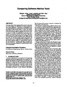
2: Data Description The data used in this study were obtained from 27 moderate-sized projects developed in a software engineering course at the University of Bari. The software represents information systems for a publishing company, based on a same specification but developed by different three person-teams over a period of 4-10 months. The systems range in size from 1100 to 9400 lines of Pascal source code. There were between 120 and 340 software components in each system, ranging in size from 60 to 530 lines of code. The term software component refers to functional abstractions of code such as procedures, functions and main programs. From each system, we randomly selected a group of 4-5 components for a total of 118 components. Each group of component was tested by independent student teams of an advanced software engineering course with the aim to find faults. The distribution of faults, shown in Figure 1, is heavily skewed in favor of components with no faults or only one fault. In order to build unbiased classification models, we decided to have an approximately equal number of components in the classes of reliability. Thus, we defined as high-risk any 60 50 40 30 20 10 0 0
1
2
3
4
5
6
7
8
9
10
11
12
13
Number of faults
Figure 1. Distribution of faults per software component
14
15
The set of 118 observations was subsequently divided into two groups. Two thirds of the components, made up of 79 observations, were randomly selected to create and tune the predictive models. The remaining 39 observations provided the data to test the models and compare their performances. From now on, the first group of observations will be called training set, while the second one testing set.
3: Implementing the Predictive Models There are many ways to build a predictive model using a given modeling technique. We describe our implementation choices to make it possible the replication of the experiment in other environments and the improvement in the application of the techniques.
3.1: Principal component analysis Most linear modeling applications, such as regression and discriminant analysis, can produce unstable models when the independent variables have a strong relationship between themselves. In this cases, principal component analysis can be used to reduce the dimensions of the metric space and obtain a smaller number of orthogonal domain metrics [8]. In our experiment, the principal component analysis applied on the 11 complexity metrics revealed three distinct complexity domains, having eigenvalues greater than 0.9. In Table 1, each column shows the degree of relationship between the 11 complexity metrics and the three orthogonal domains.
Metric V N LOC NCLOC N2 v(G) η2 fanout IF fanin DC Eigenvalues
Domain 1 0.98338 0.98209 0.97486 0.97448 0.95392 0.87488 0.73870 0.16845 -0.01610 0.12539 -0.07395 6.306010
Domain 2 0.07621 0.09208 0.07603 0.06976 0.11957 0.19214 0.01342 0.88696 0.85161 0.82472 -0.06408 2.102089
Table 1. Rotated factor pattern
Domain 3 -0.04700 -0.04874 -0.02989 -0.05521 -0.06178 -0.01642 -0.00998 0.01091 0.02215 -0.12569 0.99215 0.980321
3.2: Discriminant analysis Discriminant analysis develops a discriminant function or classification criterion to place each observation into one of mutually exclusive groups [8]. It requires that there exists a prior knowledge of the classes, in our case low-risk and high-risk components. To develop the classification criterion, we used a parametric method which uses a measure of generalized square distance and is based on the pooled covariance matrix. Using the generalized square distance, a posterior probability of an observation belonging to one of the two groups is computed. An observation is classified into the group with the greatest probability of membership. We built two different discriminant models. The first one, applying discriminant analysis directly on the original 11 complexity metrics. The second one, using as input the domain metrics obtained from the principal component analysis.
3.3: Logistic regression Logistic regression refers to an analysis which computes the probability of class membership according to the following equation [1]: n p log = c0 + ∑ ci ∗ xi 1- p i=1
where p is the probability of a software component to be high-risk, and the independent variables xi are the complexity metrics. The regression coefficients ci are computed through a maximum-likelihood estimation. Like discriminant analysis, two regression models were built. The first one is based on the original complexity measures, while the second one uses the domain metrics which have been generated from the principal component analysis.
3.4: Logical classification models Logical classification models are classifiers which can be expressed as decision trees or sets of production rules. They are generated through a recursive algorithm that selects metrics which best discriminate between components within a target class and those outside it. We used the C4.5 system [26] which is a variation on the ID3 system [25] to automatically build the classification model. C4.5 partitions continuous attributes finding the best threshold among the set of training cases. The recursive partition method continues to subdivide the
training set until each subset in the partition contains cases of a single class, or until no test offers any improvement. The result was a decision tree with 12 levels composed of 11 decision nodes and 12 leaf nodes. To achieve the goal of understandability, the decision tree was transformed in a collection of rules by removing the conditions that did not seem helpful for discriminating between classes and by excluding rules that did not contribute to the accuracy of the set of rules as a whole. This process lead to a production rule classifier made up of 12 rules ranging from 1 to 5 compound conditions. The Halstead’s metrics (η2, N2, N, V) did not appeared neither in the decision tree nor in the production rules.
3.5: Layered neural networks We used a typical feed-forward neural network [27], characterized in our experiment by one input layer of 11 neurons, each connected to a complexity metric, one output layer of only 1 neuron that sends externally the predicted risk, and one layer of 50 hidden neurons. Among the supervised algorithms we chose the most popular one, the back-propagation algorithm, which adjusts network weights by iteration until an error tolerance, defined by the user, is achieved or a maximum number of iterations have been completed. The network weights were initially set to random values between -1.0 and 1.0 using a sigmoid distribution. We trained the network with a value of 0.1 for the error tolerance, 1 for the learning rate, and 0.7 for the momentum rate. We stopped the training after 9000 iterations with 78 recognized observations over 79. The network’s input and output is bounded between 0 and 1. Thus, we reduced input data using a direct scaling. When testing the network, we increased the error tolerance to 0.5 so that low-risk components correspond to observations with an output value in the first half of [0, 1], and high-risk components to observations with an output value in the second half.
3.6: Holographic networks With holographic networks information is encoded inside holographic neurons rather than in the connection weights between neurons [32]. A holographic neuron holds a correlation matrix which enables memorizing stimulus-response associations. Individual associations are learned deterministically on one non-iterative transformation. Holographic neurons internally work with complex numbers in polar notation so that the magnitude (from 0.0 to 1.0) is interpreted as the
confidence level of data, and the phase (from 0 to 2π) serves as actual value of data. In our experiment, input data were converted to the range [0, 2π] using a sigmoid function and interpreted as phase orientation of complex values with a unity magnitude. On the contrary, the response was converted using a linear interpolation. These conversion methods provided the maximum symmetry in the distribution of data. We trained the network so to obtain a maximum error of 0.1 for each observation.
4: Evaluation Criteria To provide a sound and efficient basis for comparison, we give a set of evaluation criteria which are general enough to be applied to all types of modeling techniques used in this study. We have selected statistical criteria which are based on the analysis of categorical data. In our study we have two variables (real risk and predicted risk) that can assume only two discrete values (low and high) in a nominal scale. Then the data can be represented by a two-dimensional contingency table, shown in Table 2, which has one row for each level of variable real risk and one column for each level of variable predicted risk. The intersections of rows and columns contain the frequency of observations (nij) corresponding to the combination of variables. Row totals (ni·) and column totals (n·j) correspond to the frequency of observations for each of the variables. In our context, the first row contains low-risk components, i.e. with no faults, while the second row contains high-risk components, including at least one fault. The first column contains components which the models classifies as low-risk, while the second column contains components classified as high-risk. Predicted Risk Real Risk
low
high
low
n11
n12
n1•
high
n21
n22
n2•
n•1
n•2
n
Table 2. Two-dimensional contingency table The evaluation criteria are predictive validity, misclassification rate, achieved quality and verification cost. We use the criterion of predictive validity for assessment, since we determine the absolute worth of a predictive model by looking at its statistical significance.
A model which does not meet the criterion of predictive validity should be rejected. The remaining criteria are used for comparison, taking into account that the choice between the accepted models depend from the perspective of the software engineering manager. In practice he could be more interested in achieving a better quality at a high verification cost or be satisfied of a lower quality, sparing verification effort.
4.1: Predictive validity The predictive validity is the capability of the model to predict the future component behavior from present and past behavior. The present and past behavior is represented by data in the training set while the future behavior of components is described by data in the testing set. In our context, where data are represented by a contingency table, we apply the predictive validity by testing the null hypothesis of no association between the row variable (real risk) and the column variable (predicted risk). In this case, the predictive model is not able to discriminate low-risk components from high-risk components. The alternative hypothesis is one of general association. A chi-square (χ2) statistic [7] with a distribution of one degree of freedom is applied to test the null hypothesis.
4.2: Misclassification rate
4.3: Quality achieved We are interested in measuring how effective are the predictive models in terms of the quality achieved after that the components classified as high-risk have been undergone to a verification activity. We suppose that the verification will be so exhaustive to find the faults of all the components which are actually high-risk. We measure this criterion using the completeness measure [5], which is the percentage of faulty components that have been actually classified as such by the model. · Completeness: C = n22 / n2·
4.4: Verification cost Quality is achieved by increasing the cost of verification due to an extra effort in inspection and testing for the components which have been flagged as high-risk. We measure the verification cost by using two indicators. The former, inspection [29], measures the overall cost by considering the percentage of components which should be verified. The latter, wasted inspection, is the percentage of verified components which do not contain faults because they have been incorrectly classified. · Inspection: I = n·2 / n · Wasted Inspection: WI = n12 / n·2
5: Analysis of the Results For our predictive models, which classify components as either low-risk or high-risk, two misclassification errors are possible. A Type 1 error is made when a high-risk component is classified as lowrisk, while a Type 2 when a low-risk component is classified as high-risk. It is desirable to have both types of error small. However, since the two types of errors are not independent, software engineering managers should consider their different implications. As a result of Type 1 error, a component actually being high-risk could pass the quality control. This would cause the release of a lower quality product and more fix effort when a failure will happen. As a result of Type 2 error, a component actually being low-risk will receive more testing and inspection effort than needed. This would cause a waste of effort. In the contingency table, the number of Type 1 and Type 2 errors is given, respectively, by n21 and n12. We adopt from [29] the following measures of misclassification: · Proportion of Type 1: P1 = n21 / n · Proportion of Type 2: P2 = n12 / n · Proportion of Type 1 + Type 2: P12 = (n21 + n12) / n
We applied the evaluation criteria on the testing set and analyzed the resulting data. Table 3 shows the chisquare values and the significance levels across the predictive models built using different modeling techniques. From the low values of chi-square and high significance levels in the testing set, we accept the null hypothesis of no association between predicted risk and real risk. In fact, all the values of significance are too high with respect to the most common values which are used to reject the null hypothesis. As regards the misclassification rate, we recall that a casual prediction should have 50 percent of proportion of Type 1 + Type 2, and 25 percent for both proportion of Type 1 and Type 2. From Table 4, showing the misclassification rates, we see that the proportion of Type 1 + Type 2 error ranges between 46 percent and 59 percent. Discriminant analysis and logistic regression, when applied in conjunction with principal component analysis, have a high proportion of Type 2 error (respectively 41 and 46 percent) with respect to the proportion of Type 1 error (respectively 15 and 13 percent). On the contrary, the other models have
balanced values of Type 1 and Type 2 error, ranging between 20 and 28 percent. Looking at Table 5, we can interpret better the misclassification results. In fact, the highest values of quality correspond to the models built with principal component analysis followed from either discriminant analysis or logistic regression (completeness is, respectively, 68 and 74 percent). But these high values of quality are obtained by inspecting the great majority of components (inspection is, respectively, 74 and 82 percent), thus wasting more than one half of the verification effort (wasted inspection is, respectively, 55 and 56 percent). The lowest level of quality (completeness is 42 percent) is achieved by both discriminant analysis and logistic regression, when used without principal component analysis, and by the layered neural network. The logistic regression without principal components and the layered neural network have also the poorest results in correctly identifying the high-risk components (wasted inspection is 58 percent). On the contrary the logical classification model is the only model which dissipates less than one half of the verification effort (wasted inspection is 47 percent). Modeling Techniques Discriminant analysis Discriminant analysis with Principal components Logistic regression Logistic regression with Principal components Logical classification model Layered neural network Holographic network
χ2 0.244 0.685
α 0.621 0.408
0.648 1.761
0.421 0.184
0.215 0.648 0.227
0.643 0.421 0.634
Table 3. Evaluation of predictive validity Modeling Techniques Discriminant analysis Discriminant analysis with Principal components Logistic regression Logistic regression with Principal components Logical classification model Layered neural network Holographic network
P1 28.21 15.38
P2 25.64 41.03
P12 53.85 56.41
28.21 12.82
28.21 46.15
56.41 58.97
25.64 28.21 25.64
20.51 28.21 28.21
46.15 56.41 53.85
Table 4. Evaluation of misclassification rate
Modeling Techniques Discriminant analysis Discriminant analysis with Principal components Logistic regression Logistic regression with Principal components Logical classification model Layered neural network Holographic network
C 42.11 68.42
I 46.15 74.36
WI 55.56 55.17
42.11 73.68
48.72 82.05
57.89 56.25
47.37 42.11 47.37
43.59 48.72 51.28
47.06 57.89 55.00
Table 5. Evaluation of achieved quality and verification cost
6: Conclusions This paper has presented an analysis of classification models predicting quality classes on the basis of software complexity measures. The models used in this study, were based on various classification paradigms such as statistical analysis, machine learning and neural networks. Despite of this variegated selection of modeling techniques, no model satisfies the criterion of predictive validity, that is no model is able to discriminate between components with faults and components without faults. This result is in contrast with various papers which report successful results in recognizing fault-prone components from analogous sets of complexity measures. Briand et al. [6] presented an experiment for predicting high-risk components using two logical classification models (Optimized Set Reduction and classification tree) and two logistic regression models (with and without principal components). Design and code metrics were collected from 146 components of a 260 KLOC system. OSR classifications were found to be the most complete (96 percent) and correct (92 percent), where correctness is the complement of our wasted inspection. The classification tree was more complete (82 percent) and correct (83 percent) than logistic regression models. The use of principal components improved the accuracy of logistic regression, from 67 to 71 percent of completeness and from 77 to 80 percent of correctness. Porter [24] presented an application of classification trees to data collected from 1400 components of six FORTRAN projects in NASA environment. For each component, 19 attributes were measured, capturing information spanning from design specifications to implementation. He measured the mean accuracy across all tree applications according to completeness (82
percent) and to the percentage of components whose target class membership is correctly identified (72 percent), that is the complement of the Proportion of Type 1 and Type 2 error. Munson and Koshgoftaar [22] detected faulty components by applying principal component analysis and discriminant analysis to discriminate between programs with less than five faults and programs having 5 or more faults. The data set included 327 program modules from two distinct Ada projects of a command and control communication system. They collected 14 metrics, including Halstead’s metrics together with other code metrics. Applying discriminant analysis with principal components, at a probability level of 80 percent, resulted in recognizing 79 percent of the modules with a total misclassification rate of 5 percent. Our result is closer with the investigation performed by Basili and Perricone [2], where the unexpected result was that module size and cyclomatic complexity had no relationship with the number of faults, although there was a negative relationship with the fault density. From our study, we argue that the relationship between software complexity measures and software quality cannot be considered an assumption which holds for any data set and project, but should be validated in each specific environment [3], [28]. A predictive model, from the simplest to the most complex, is worthwhile only if there is a local process to select metrics which are valid as predictors. Another unexpected result in our study has been obtained from reducing the complexity metrics to three principal components before to apply discriminant analysis or logistic regression. The good performance in achieved quality is exclusively the result of classifying very often components to be high-risk. Further work is underway to find software complexity metrics which are best related to our fault data and to expand the scope of the modeling techniques.
Acknowledgements We would like to thank Fabio Abbattista and Donato Malerba of the University of Bari for providing useful comments and suggestions. Also, we wish to thank Giulia Festino for her support in processing and analyzing the data. Finally, we thank students from the University of Bari for providing the fault data used in this study.
References [1] [2]
[3]
[4]
[5]
[6]
[7] [8]
[9]
[10] [11]
[12] [13]
[14]
A. Agresti, Categorical Data Analysis, John Wiley & Sons, New York, 1990. V. R. Basili, and B. T. Perricone, “Software errors and complexity: an empirical investigation”, Communications of the ACM, vol.27, no.1, January 1984, pp.42-52. V. R. Basili, and H. D. Rombach, “The TAME project: towards improvement-oriented software environments”, IEEE Transactions on Software Engineering, vol.14, no.6, June 1988, pp.758-773. G. Boetticher, K. Srinivas, and D. Eichmann, “A neural net-based approach to software metrics”, in Proceedings of the 5th International Conference on Software Engineering and Knowledge Engineering, San Francisco, California, June 1993, pp.271-274. L. C. Briand, W. M. Thomas, and C. J. Hetmanski, “Modeling and managing risk early in software development”, in Proceedings of the 15th International Conference on Software Engineering, Baltimore, Maryland, May 1993, pp.55-65. L. C. Briand, V. R. Basili, and C. J. Hetmanski, “Developing interpretable models with optimized set reduction for identifying high-risk software components”, IEEE Transactions on Software Engineering, vol.19, no.11, November 1993, pp.1028-1044. W. J. Conover, Practical Nonparametric Statistics, Wiley, New York, 1971. W. R. Dillon, and M. Goldstein, Multivariate Analysis: Methods and Applications, John Wiley & Sons, New York, 1984. J. C. Esteva, and R. G. Reynolds, “Identifying reusable software components by induction”, International Journal of Software Engineering and Knowledge Engineering, vol.1, no.3, 1991, pp.271292. N. E. Fenton, Software Metrics: A Rigorous Approach, Chapman & Hall, London, 1991. A. Fitzsimmons, and T. Love, “A review and evaluation of software science”, Computing Surveys, vol.10, no.1, March1978, pp.3-18. M. H. Halstead, Elements of Software Science, Elsevier North-Holland, New York, 1977. S. Henry, and D. Kafura, “Software structure metrics based on information flow”, IEEE Transactions on Software Engineering, vol.SE-7, no.5, September 1981, pp.510-518. G. Jensen, “Quality control in manufacturing based on fuzzy classification”, in Frontier Decision
[15]
[16]
[17]
[18]
[19]
[20]
[21]
[22]
[23]
[24]
[25]
Support Concepts, John Wiley & Sons, New York, 1994, pp.107-118. N. Karunanithi, D. Whitley, and Y. K. Malaiya, “Prediction of software reliability using connectionists models”, IEEE Transactions on Software Engineering, vol.18, no.7, July 1992, pp.563-573. N. Karunanithi, D. Whitley, and Y. K. Malaiya, “Using neural networks in reliability prediction”, IEEE Software, July 1992, pp.53-59 T. M. Khoshgoftaar, D. L. Lanning, and J. C. Munson, “A comparative study of predictive models for program changes during system testing and maintenance”, in Proceedings of the Conference on Software Maintenance, Montreal, Canada, September 1993, pp.72-79. T. M. Khoshgoftaar, and R. M. Szabo, “Improving code churn prediction during the system test and maintenance phases”, in Proceedings of the International Conference on Software Maintenance, Victoria, British Columbia, Canada, September 1994, pp.58-67. F. Lanubile, and G. Visaggio, “Quality evaluation on software reengineering based on fuzzy classification”, in Frontier Decision Support Concepts, John Wiley & Sons, New York, 1994, pp.119-134. J. Lewis, amd S. Henry, “A methodology for integrating maintainability using software metrics”, in Proceedings of the Conference on Software Maintenance, Miami, FL, October 1989, pp.32-39. T. J. McCabe, “A complexity measure”, IEEE Transactions on Software Engineering, vol.SE-2, no.4, December 1976, pp.308-320. J. C. Munson, and T. M. Khoshgoftaar, “The detection of fault-prone programs”, IEEE Transactions on Software Engineering, vol.18, no.5, May 1992, pp.423-433. A. A. Porter, and R. W. Selby, “Empirically guided software development using metric-based classification trees”, IEEE Software, March 1990, pp.46-54. A. A. Porter, “Developing and analyzing classification rules for predicting faulty software components”, in Proceedings of the 5th International Conference on Software Engineering and Knowledge Engineering, San Francisco, California, June 1993, pp.453-461. J. R. Quinlan, “Induction of decision trees”, Machine Learning, vol.1, no.1, 1986, pp.81-106.
[26] J. R. Quinlan, C4.5: Programs for Machine Learning, Morgan Kauffman Publishers, San Mateo, CA, 1993. [27] D. Rumelhart, G. Hinton, and R. Williams, “Learning internal representations by error propagation”, in Parallel Distribuited Processing, vol.I, MIT Press, Cambridge, MA, 1986, pp.318362. [28] N. F. Schneidewind, “Methodology for validating software metrics”, IEEE Transactions on Software Engineering, vol.18, no.5, May 1992, pp.410-422. [29] N. F. Schneidewind, “Validating metrics for ensuring Space Shuttle Flight software quality”, Computer, August 1994, pp.50-57. [30] R. W. Selby, and A. A. Porter, “Learning from examples: generation and evaluation of decision trees for software resource analysis”, IEEE Transactions on Software Engineering, vol.14, no.12, December 1988, pp.1743-1757. [31] B. Soucek, J. Sutherland, and G. Visaggio, “Holographic decision support system: credit scoring based on quality metrics”, in Frontier Decision Support Concepts, John Wiley & Sons, New York, 1994, pp.171-182. [32] J. Sutherland, “A holographic model of memory, learning and expression”, International Journal of Neural Systems, vol.1, no.3, 1990, pp.259-267.