Comparing Robot Controllers. Through System Identification. Ulrich Nehmzow1, Otar Akanyeti1, Roberto Iglesias2,. Theocharis Kyriacou1, and S.A. Billings3.
Comparing Robot Controllers Through System Identification Ulrich Nehmzow1 , Otar Akanyeti1 , Roberto Iglesias2 , Theocharis Kyriacou1, and S.A. Billings3 1
Department of Computer Science, University of Essex, UK 2 Electronics and Computer Science, University of Santiago de Compostela, Spain 3 Dept. of Automatic Control and Systems Engineering, University of Sheffield, UK
Abstract. In mobile robotics, it is common to find different control programs designed to achieve a particular robot task. It is often necessary to compare the performance of such controllers. So far this is usually done qualitatively, because of a lack of quantitative behaviour analysis methods. In this paper we present a novel approach to compare robot control codes quantitatively, based on system identification. Using the NARMAX system identification process, we “translate” the original behaviour into a transparent, analysable mathematical model of the original behaviour. We then use statistical methods and sensitivity analysis to compare models quantitatively. We demonstrate our approach by comparing two different robot control programs, which were designed to drive a Magellan Pro robot through door-like openings.
1
Introduction
In mobile robotics it is common to find different control programs, developed for the same behaviour, typically developed through an empirical trial-and-error process of iterative refinement. It is often interesting to compare and analyse such different controllers for the same behaviour. However, because of a lack of quantitative descriptors of behaviour such analyses are usually qualitative. As the number of controllers developed for identical tasks increases, the need for fair comparisons based on quantitative measures also becomes more important, and to find quantitative answers to questions like “What are the advantages and disadvantages of each controller?”, “Which one is more stable and efficient?”, “Will they work in completely different environments or crash even with slight modifications?” will enhance our understanding of robot-environment interaction. Realistic mobile robot control programs tend to be so complex that their direct analysis is impossible — the “meaning” of thousands of lines of code is not clear to a human observer. In this paper we therefore propose the alternative approach of “identifying” the behaviour in question, using transparent polynomial models S. Nolfi et al. (Eds.): SAB 2006, LNAI 4095, pp. 840–851, 2006. c Springer-Verlag Berlin Heidelberg 2006 �
Comparing Robot Controllers Through System Identification
841
obtained through NARMAX system identification [1], to ascertain the validity of the model, and to analyse the model instead of the original behaviour, both qualitatively and quantitatively.
2
Controller Identification
Motivation and Related Work. The main benefits of “system identification” (i.e. mathematical modelling) are 1. Efficiency: The obtained models are polynomials. They are fast in execution and occupy little space in memory. 2. Transparency: The transparent model structure simplifies mathematical analysis 3. Portability: Polynomial models are universal, in the sense that they can be quickly incorporated into any robot programming language. Our models are obtained based on NARMAX (Nonlinear Auto-Regressive Moving Average model with eXogenous inputs) system identification [1]. This identification process has already been applied in modelling sensor-motor couplings of robot controllers [2, 4]. In [5] we demonstrate how easy it is to exchange the generated models between different robot platforms. After the identification of the controllers it is relatively straightforward to evaluate the models and to compare them quantitatively. The work presented in [3] gives examples of the characterisation of models of robot behaviour. The system identification process can be divided into two stages: First the robot is driven by the original robot controller which we wish to analyse. While the robot is moving, we log sensor and motor information to model the relationship between the robot’s sensor perception and motor responses. In the second stage, a nonlinear polynomial NARMAX model (see below) is estimated. This model relates input sensor values to output actuator signals and subsequently can be used to control the robot. NARMAX Modelling. The NARMAX modelling approach is a parameter estimation methodology for identifying the important model terms and associated parameters of unknown nonlinear dynamic systems. For multiple input, single output noiseless systems this model takes the form: y(n) = f (u1 (n), u1 (n − 1), u1 (n − 2), · · · , u1 (n − Nu ), u1 (n)2 , u1 (n − 1)2 , u1 (n − 2)2 , · · · , u1 (n − Nu )2 , · · · , u1 (n)l , u1 (n − 1)l , u1 (n − 2)l , · · · , u1 (n − Nu )l , u2 (n), u2 (n − 1), u2 (n − 2), · · · , u2 (n − Nu ), u2 (n)2 , 2
2
2
l
l
u2 (n − 1) , u2 (n − 2) , · · · , u2 (n − Nu ) , · · · , u2 (n) , u2 (n − 1) , u2 (n − 2)l , · · · , u2 (n − Nu )l , · · · , ud (n), ud (n − 1), ud (n − 2), · · · , ud (n − Nu ), ud (n)2 , ud (n − 1)2 , ud (n − 2)2 , · · · , ud (n − Nu )2 , · · · , ud (n)l , ud (n − 1)l , ud (n − 2)l , · · · , ud (n − Nu )l , y(n − 1), y(n − 2), · · · , 2
2
2
l
y(n − Ny ), y(n − 1) , y(n − 2) , · · · , y(n − Ny ) , · · · , y(n − 1) , l
l
y(n − 2) , · · · , y(n − Ny ) )
842
U. Nehmzow et al.
where y(n) and u (n) are the sampled output and input signals at time n respectively, Ny and Nu are the regression orders of the output and input respectively and d is the input dimension. f () is a non-linear function, this is typically taken to be a polynomial or wavelet multi-resolution expansion of the arguments. The degree l of the polynomial is the highest sum of powers in any of its terms. The NARMAX methodology breaks the modelling problem into the following steps: i) structure detection, ii) parameter estimation, iii) model validation, iv) prediction and v) analysis. Logged data is first split into two sets (usually of equal size). The first, the estimation data set, is used to determine model structure and parameters. The remaining data set, the validation data set, is subsequently used to validate the model.
3
Experimental Scenario: Door Traversal
The example presented in this paper demonstrates how system identification can be used to model sensor-motor couplings of two different robot controllers designed to achieve the same particular task: the episodic task of “door traversal”, where each episode comprises the movement of the robot from a starting position to a final position, traversing a door-like opening en route. In this paper, we compare two different controllers for this task. “Model 1” is a hard-wired laser controller which maps the laser perception of the robot onto action, using a behaviour based approach. For “model 2”, the robot was driven manually by a human operator. While these two original behaviours were being executed, we logged all sensory perceptions, motor responses and the robot’s precise position, using a camera logging system, every 160 ms. 300cm 300cm
60cm
60cm
80cm
(a)
(b)
80cm
(c)
Fig. 1. The Magellan Pro robot used in the experiments (a). Training environments for the “Hard-Wired Laser Controller” (model 1, centre) and “Manual Control” (model 2, right). Environment (b) has extra walls on the wings of the door-like opening. The initial positions of the robot were within the shaded area indicated in each figure; door openings were twice the robot’s diameter (80cm).
Comparing Robot Controllers Through System Identification
843
Each controller was then modelled through non-linear polynomial functions (NARMAX), so that the resulting two models identify the two robot controllers by relating robot perception to action. To test the validity of the two models, we then let the models themselves control the robot. The models of the two different robot controllers were deliberately trained in different environments (figure 1 (b,c)), with different translational velocities and different sensor information, to simulate the natural differences which might exist between different implementations of the same task. All experiments were conducted with a Magellan Pro robot (figure 1 (a)) in the Robotics Arena at Essex University. 3.1
Model 1: Hardwired Laser Control
The first control program used a hardwired, behaviour-based control strategy that mapped laser perception to steering speed of the robot. The translational velocity of robot was kept constant at 0.2 m/s, the laser perception of the robot was encoded in 36 sectors by taking the median value of every 5 degree interval over a semi-circle. The model of the robot’s angular velocity ω, obtained through NARMAX system identification, contains 84 terms and is given in table 1. Table 1. Model 1: NARMAX model of the angular velocity ω as a function of laser perception for the “hard-wired laser controller”. d1 , · · · , d29 are laser bins, coarse coded by taking the median value over each 5-degree interval. ω = 0.574 + 0.045 ∗ d1 (t) + 0.001 ∗ d6 (t) + 0.032 ∗ d7 (t) − 0.017 ∗ d8 (t) +0.113 ∗ d9 (t) − 0.099 ∗ d10 (t) − 0.011 ∗ d11 (t) − 0.006 ∗ d12 (t) − 0.020 ∗ d13 (t) +0.020 ∗ d14 (t) − 0.015 ∗ d15 (t) − 0.016 ∗ d16 (t) − 0.046 ∗ d20 (t) − 0.009 ∗ d21 (t) +0.007 ∗ d22 (t) − 0.035 ∗ d23 − 0.017 ∗ d24 (t) − 0.056 ∗ d25 (t) + 0.026 ∗ d26 (t) +0.039 ∗ d27 (t) − 0.003 ∗ d28 (t) + 0.044 ∗ d29 (t) − 0.018 ∗ d30 (t) − 0.144 ∗ d31 (t) +0.001 ∗ d32 (t) − 0.023 ∗ d21 (t) − 0.001 ∗ d26 (t) − 0.011 ∗ d27 (t) + 0.003 ∗ d28 (t) −0.010 ∗ d213 (t) − 0.001 ∗ d215 (t) − 0.005 ∗ d216 (t) − 0.001 ∗ d217 (t) −0.002 ∗ d219 (t) + 0.002 ∗ d220 (t) − 0.001 ∗ d221 (t) − 0.001 ∗ d222 (t) +0.002 ∗ d223 (t) + 0.002 ∗ d224 (t) + 0.008 ∗ d225 (t) − 0.004 ∗ d227 (t) −0.001 ∗ d228 (t) + 0.019 ∗ d231 (t) − 0.001 ∗ d235 (t) + 0.001 ∗ d236 (t) −0.001 ∗ d1 (t) ∗ d7 (t) − 0.001 ∗ d1 (t) ∗ d18 (t) + 0.001 ∗ d1 (t) ∗ d20 (t) +0.003 ∗ d1 (t) ∗ d22 (t) + 0.006 ∗ d1 (t) ∗ d23 (t) − 0.003 ∗ d1 (t) ∗ d25 (t) −0.001 ∗ d1 (t) ∗ d32 (t) + 0.003 ∗ d1 (t) ∗ d33 (t) + 0.007 ∗ d1 (t) ∗ d34 (t) −0.002 ∗ d1 (t) ∗ d36 (t) + 0.003 ∗ d7 (t) ∗ d16 (t) − 0.001 ∗ d8 (t) ∗ d10 (t) −0.006 ∗ d9 (t) ∗ d14 (t) − 0.003 ∗ d9 (t) ∗ d17 (t) − 0.009 ∗ d9 (t) ∗ d18 (t) −0.002 ∗ d9 (t) ∗ d28 (t) + 0.013 ∗ d10 (t) ∗ d13 (t) − 0.002 ∗ d11 (t) ∗ d16 (t) +0.004 ∗ d11 (t) ∗ d18 (t) − 0.001 ∗ d12 (t) ∗ d15 (t) + 0.001 ∗ d12 (t) ∗ d16 (t) +0.002 ∗ d12 (t) ∗ d18 (t) + 0.002 ∗ d13 (t) ∗ d15 (t) + 0.011 ∗ d13 (t) ∗ d16 (t) −0.003 ∗ d14 (t) ∗ d16 (t) + 0.002 ∗ d14 (t) ∗ d23 (t) + 0.001 ∗ d14 (t) ∗ d36 (t) +0.002 ∗ d15 (t) ∗ d21 (t) + 0.003 ∗ d16 (t) ∗ d19 (t) + 0.002 ∗ d16 (t) ∗ d25 (t) +0.002 ∗ d17 (t) ∗ d28 (t) + 0.001 ∗ d18 (t) ∗ d31 (t) + 0.001 ∗ d20 (t) ∗ d21 (t) +0.002 ∗ d20 (t) ∗ d28 (t) + 0.003 ∗ d20 (t) ∗ d31 (t) − 0.004 ∗ d21 (t) ∗ d26 (t) +0.005 ∗ d21 (t) ∗ d30 (t) − 0.005 ∗ d25 (t) ∗ d29 (t)
844
U. Nehmzow et al.
Qualitative Model Evaluation. Figure 2 shows the trajectories of the robot under the control of the original hard-wired laser controller and its NARMAX model respectively. In both cases the robot was started from 36 different initial positions, and completed the task successfully in each case.
(a)
(b)
Fig. 2. Robot trajectories under control by the original “Hard-wired Laser Controller” (a) and under control by its model, “model 1” (b). Note that side walls of the environment can not be seen in the figures because they were outside the field of view of the camera.
3.2
Model 2: Manual Control
The second control strategy used was to drive the robot through the opening manually. Here, the translational velocity of robot was kept constant at 0.07 m/s. For sensor information (i.e. model input), the values delivered by the laser scanner were averaged in twelve sectors of 15 degrees each, to obtain a twelve dimensional vector of laser distances. These laser bins as well as the 16 sonar sensor values were inverted before they were used to obtain the model, so that large readings indicate close-by objects. The identified model of the angular velocity ω, which contained 35 terms, is given in table 2. Qualitative Model Evaluation. Figure 3 shows the trajectories of the robot under the control of human operator and its NARMAX model respectively. In both cases the robot was started with 41 different initial positions, and passed through the door-like gap successfully each time.
4
Comparison of the Two Models
Figures 2 and 3 show that on a qualitative level both models are good representations of the original. Small differences in trajectory between “original” and “model-controlled” behaviour we attribute to natural fluctuations in robotenvironment interaction.
Comparing Robot Controllers Through System Identification
845
Table 2. Model 2: NARMAX model of the angular velocity ω as a function of sensor perception for the door traversal behaviour under manual control. s10 , · · · , s16 are the inverted and normalised sonar readings (s�i = (1/si − 0.25)/19.75), while d1 , · · · , d6 are the inverted and normalised laser bins d�i = (1/di − 0.12)/19.88. Taken from [4]. ω(t) = 0.010 − 1.633 ∗ d�1 (t) − 2.482 ∗ d�2 (t) + 0.171 ∗ d�3 (t) + 0.977 ∗ d�4 (t) � −1.033 ∗ d�5 (t) + 1.947 ∗ d�6 (t) + 0.331 ∗ s�13 (t) − 1.257 ∗ s�15 (t) + 12.639 ∗ d12 (t) � � � 2 2 2 � � +16.474 ∗ d2 (t) + 28.175 ∗ s15 (t) + 80.032 ∗ s16 (t) + 14.403 ∗ d1 (t) ∗ d3 (t) −209.752 ∗ d�1 (t) ∗ d�5 (t) − 5.583 ∗ d�1 (t) ∗ d�6 (t) + 178.641 ∗ d�1 (t) ∗ s�11 (t) −126.311 ∗ d�1 (t) ∗ s�16 (t) + 1.662 ∗ d�2 (t) ∗ d�3 (t) + 225.522 ∗ d�2 (t) ∗ d�5 (t) −173.078 ∗ d�2 (t) ∗ s�11 (t) + 25.348 ∗ d�3 (t) ∗ s�12 (t) − 24.699 ∗ d�3 (t) ∗ s�15 (t) +100.242 ∗ d�4 (t) ∗ d�6 (t) − 17.954 ∗ d�4 (t) ∗ s�12 (t) − 3.886 ∗ d�4 (t) ∗ s�15 (t) −173.255 ∗ d�5 (t) ∗ s�11 (t) + 40.926 ∗ d�5 (t) ∗ s�15 (t) − 73.090 ∗ d�5 (t) ∗ s�16 (t) −144.247 ∗ d�6 (t) ∗ s�12 (t) − 57.092 ∗ d�6 (t) ∗ s�13 (t)) + 36.413 ∗ d�6 (t) ∗ s�14 (t) −55.085 ∗ s�11 (t) ∗ s�14 (t) + 28.286 ∗ s�12 (t) ∗ s�15 (t) − 11.211 ∗ s�14 (t) ∗ s�16 (t)
(a)
(b)
Fig. 3. Robot Trajectories under under “manual control” (a) and under control of its model, “model 2” (b). Taken from [4].
It is interesting to see that “Model 1” has significantly more terms (83) than “Model 2” (35), and therefore requires more memory and computing power resources. Immediately obvious is also that model 2 is simpler, in that it only uses information from sensors found on the right side of the robot. In the following, we were interested in investigating the differences between the models of the two door-traversal behaviours further. Testing and Evaluation Setup. We first tested the controllers in four different environments (figure 4) to reveal differences in the behaviour of the robot when controlled by the two models. To minimise the influence of constant errors, model 1 and model 2 were selected randomly to control the robot. In the first scenario (figure 4 (1)), the robot was driven by “Model 1” in the training environment of “Model 2”. After this, the two controllers were tested in a completely different environment, where two door-like openings with equal
846
U. Nehmzow et al.
80cm
80cm
80cm
80cm
(1)
(2)
(3)
(4)
Fig. 4. Four different test environments used to compare the two models qualitatively. 1) Single-door test scenario, 2) Double-door test scenario, 3) Completely-enclosed test scenario, 4) Enclosure with a single door. The initial positions of the robot are within the shaded area indicated in each figure. All openings found in the environment had a width of two robot diameters (80cm).
width were presented at the same time (figure 4 (2)). This demonstrated how each opening interfered with the robot’s behaviour. It also revealed the dominant sensors. In the third and fourth scenarios (figure 4 (3) and (4)) we tried to measure the effect of a gap found in an environment. We assumed that in this application openings would be the dominant environmental factors in robot-environment interaction. Therefore the models were tested first in a completely closed environment, subsequently we introduced a gap to observe the resulting change in behaviour. 4.1
Qualitative Comparison
As can be seen in figure 5, when we remove the side walls from the environment, the robot under the control of “Model 1” has some problems in centreing itself while passing through the gap. We realised that side walls make the robot turn sharper while approaching to the door-like opening, which made it easier for robot to centre itself while passing through the gap. For the double-door test scenario, it is interesting to see how two gaps interfere with each other for the behaviour of robot under the control of “Model 1”. If the robot was started from the middle region between two gaps, it generally collided with the wall, without turning towards any of the gaps. If the robot pointed at one of the gaps initially, it was attracted towards it, but the other gap still effected the behaviour and the robot could not centre itself enough to pass through the gap (figure 6 (a)). When we look at the trajectories of robot under the control of “Model 2” (figure 6 (b)), we observe that the two gaps do not interfere with each other. This is a predictable outcome, as “Model 2” uses sensors only from the right side of the robot. Therefore, if the robot detects the gap found on the right side, it
Comparing Robot Controllers Through System Identification
(a)
847
(b)
Fig. 5. Robot trajectories under the control of “Model 1” in the training environment of “Model 1” (a), and in the training environment of “Model 2” (b). The arrows in both figures indicate how much the robot deviated from the centre point of the opening while passing through it. Note that side walls of the environment in (A) can not be seen in the figure because of the limited range of camera view.
(a)
(b)
Fig. 6. Robot Trajectories in the “double door” test scenario under the control of “Model 1” (a), and controlled by “Model 2” (b).
passes through it. If it doesn’t, it automatically turns to the left, finds the other gap and traverses it. In the completely-enclosed environment, “Model 1” turned the robot constantly to the left. Figure 7 (a) shows a sample trajectory of robot under the control of “Model 1”. When we introduced a gap to the environment, we observed that the gap has the dominating effect on the controller behaviour. Although the model can not pass through the gap successfully in every trial, we still observe a general tendency of robot towards the gap (figure 7 (b)). Finally, “Model 2” showed very unstable characteristics in the last two environments. When we look at the trajectories closely we observe oscillations in
848
U. Nehmzow et al.
(a)
(b)
(c)
(d)
Fig. 7. Robot trajectories under control of “Model 1” in the “Completely enclosed environment” (a) and when an opening is introduced to the enclosed environment (b). Robot trajectories under control of “Model 2” in the “Completely enclosed environment” (c), and when an opening is introduced to the enclosed environment (d).
the robot’s behaviour, especially when the robot is close to corners. The overall model generally looks like a right wall follower when the robot is far from the corners. As it comes closer, the variation in angular velocity of the robot increases and it bumps into the corners (figure 7 (c)). We can also see that for “Model 2”, the influence of the gap on the robot behaviour is not as big as the influence on “Model 1” (figure 7 (d)). 4.2
Quantitative Comparison
When we look at the behaviours of the robot qualitatively in different test environments, we see that the responses of the two models differ. We also observe that both models do not produce a general door-traversal behaviour, but that they fail in environments that differ considerably from the training environment. In this section, we extended our work by comparing the two models quantitatively, based on a “hardware in the loop simulation” process. Hardware in the Loop Simulation. In the first quantitative analysis we wanted to see if the two models produce similar outputs for the same inputs. We
Comparing Robot Controllers Through System Identification
(a)
849
(b)
Fig. 8. Trajectory along which sensor data for “hardware in the loop” simulation was taken (a), and steering velocity graphs of both models for the given trajectory (b). There is no significant correlation between the two model’s angular velocities (rS =0.078, not sig.,p>5%). Table 3. Spearman rank correlation coefficients between “model 1” and “model 2” responses to identical real world input data Environment rS 1 0.08 2 -0.09 3 0.27 4 0.02
Stat. Sig. not sig. (p>0.05) sig. (p