EKONOMSKA ISTRAŽIVANJA-ECONOMIC RESERACH ISSN 1331-677X print 2013 Volume 26(3): 81-98
COMPARING THE BANK FAILURE PREDICTION PERFORMANCE OF NEURAL NETWORKS AND SUPPORT VECTOR MACHINES: THE TURKISH CASE Fatih Ecer a
Assistant Professor, Ph. D, Afyon Kocatepe University, Faculty of Economics and Administrative Sciences, Department of International Trade and Finance, Afyonkarahisar, Turkey,
[email protected]. a
ABSTRACT
ARTICLE INFO Article data: - Received: 28 February 2012 - Accepted: 26 September 2012 JEL classification: C38, C45, F32, N5 Keywords: - Current account - Balance of payments - ARDL - Bound Test
Experience from the banking crises during the past two decades suggest that advanced prediction models are needed for helping prevent bank failures. This paper compares the ability of artificial neural networks and support vector machines in predicting bank failures. Although artificial neural networks have widely been applied complex problems in business, the literature utilizing support vector machines is relatively narrow and their capability for predicting bank failures is not very familiar. In this paper, these two intelligent techniques are applied to a dataset of Turkish commercial banks. Empirical findings show that although the prediction performance of the two models can be considered as satisfactory, neural networks show slightly better predictive ability than support vector machines. In addition, different types of error from each model also indicate that neural network models are better predictors.
Reference to this paper should be made as follows: Ecer, F. 2013. Comparing the bank failure prediction performance of neural networks and support vector machines: The Turkish case, Ekonomska istraživanja – Economic Research 26(3):81-98 .
Copyright © 2013 Juraj Dobrila University of Pula, Department for Economics and Tourism “Dr. Mijo Mirković” http://theerjournal.com
Fatih Ecer
I. INTRODUCTION Banking is an activity that influences all the other activities and the economy as a whole. The risk of a banking crisis suggests an important need of identifying banks with potential problems even before they face severe liquidity or solvency crises. Many reasons have been denoted for bank failures including poor management practices, expanded risk-taking, inadequate accounting standards, interest rate volatility, pervasive internal control weaknesses, and increased competition from nondepository institutions (Miletić, 2008; Alam, Booth, Thordason, 2000). The last crisis has demonstrated that banks play very important role in the economy. In contrast to past crises, the current crisis began in developed countries and their economies have been influenced adversely. Unemployment has increased considerably, investments and consumption have decreased and all the governments are looking at possible ways to exit the crisis. In such cases, early warning systems help to monitor banks and prevent similar problems. Thus, the development of early warning systems is very important for regulators and policymakers. If successful, the governments could take actions to protect their markets from financial crisis, by avoiding crises in the banking sector and poor banking supervision (Ioannidis, Pasiouras, Zopounidis, 2010; Yim and Mitchell, 2004). In this paper, Turkish banking failures investigated. The Turkish economy is important to the world since Turkey has the world’s 15th largest GDP-PPP and 17th largest nominal GDP. Nowadays, the Turkish banking sector is among the strongest in Central Asia, the Middle East, and East Europe. In 2010, five Turkish banks were listed in the Forbes Global 2000 which is an annual ranking of the top 2000 public companies in the world. Eichengreen (2002) captures attention to threats coming from Turkey and Argentina. He also argues that the problems of these countries have not received sufficient attention and they must be addressed to safeguard global financial stability. Hence, we have selected Turkey as the application domain and the proposed models for failure prediction are tested for the Turkish banking sector. Turkey has a larger number of financial crises than many of the countries in the world. The Turkish banking sector was severely tested in the 1994 financial crisis and was recovered rapidly by the Turkish government. However, the Asian crises together with the two ruinous earthquakes had a negative impact on the Turkish economy and the banking sector at the end of 1990s. A November 2000 crisis led to a significant erosion of the capital base of the banking sector and exposed further the fragility of the system. The political uncertainties, the loss of credibility of the exchange rate regime, and the abolition of the exchange rate peg in February 2001 further hit the banking sector. During the November 2000 and February 2001 crises, some banks failed financially. Consequently, some banks ended their operations and some banks were taken over by the Savings Deposit Insurance Fund. The last crises affected 25 percent of the banks in Turkey and the total cost of them was estimated to be 50 billion dollars (Boyacioglu, Kara, Baykan, 2009; OzkanGunay and Ozkan, 2007). The study of bank failures is interesting because if examiners can detect problems early, regulatory actions can be taken either to minimize the cost to the governments or to prevent a bank from failing. It is therefore desirable to explore new prediction models and to provide early warnings to regulatory agencies (Thomson, 1991; Tam and Kiang, 1992). Since 1990s, artificial neural networks (ANNs) have widely been used to solve complex problems and have proven quite successful in many business applications. They can be an efficient tool to reveal critical issues in business decisions (Wu and Wang, 2000). Recently, support vector machines (SVMs) have applied complex problems in business. The SVMs have been used to financial applications such as bankruptcy prediction, credit ratings, and the detection of insurance claim fraud (Kumar and 82
COMPARING THE BANK FAILURE PREDICTION PERFORMANCE OF NEURAL NETWORKS AND SUPPORT VECTOR MACHINES: THE TURKISH CASE
Economic Research, Vol. 26 (2013) No. 3 (81-98)
Ravi, 2007). However, especially in the banking failure, the literature exploiting this approach is exiguous. The purpose of this paper is to compare the prediction performances of ANNs and SVMs for predicting Turkish banking failures. For this purpose, we implemented ANOVA test on 36 financial ratios. 22 out of 36 financial ratios were eliminated by the ANOVA and the rest 14 financial ratios were thought to be more useful in making a difference between the failed and healthy banks. Then, the data set was divided into training and validation sets. The training set and the validation set were created using the banks for one year prior to failure and two years prior to failure respectively. Both the two sets consisted of randomly chosen 34 banks in which 17 banks were failed and 17 banks were healthy. In addition, the output variable of two models is the status of banks failed or healthy. Finally, we applied different ANN models and SVMs to bank failure problem in the Turkish case and presented a comparison of the prediction performance of these models. The remainder of this paper is organized as follows: Section 2 positions the survey within the existing literature on bankruptcy forecasting studies. Section 3 briefly reviews some prediction models used in this paper. Section 4 discusses the research design including sampling and variables. Experimental results are presented in Section 5. Discussions are presented in Section 6. Finally, Section 7 summarizes our conclusions.
II. RELATED STUDIES In literature, ANNs and SVMs have been applied to solve bankruptcy problems. Both of these models are categorized into artificial intelligent models and provide examiners with more precise predictions. However, the literature on comparing these models for bank failure problems is relatively narrow in the Turkish case. Since the early 1990’s, much of the research on ANNs have focused on finance problems, with special attention to bankruptcy prediction (Du Jardin, 2010; Paliwal and Kumar, 2009). Odom and Sharda (1990) are the first researchers who used ANNs to predict the failures of firms. They developed an ANN model for bankruptcy prediction and tested using financial data from various firms. The same set of data was analyzed using multivariate discriminant analysis (MDA). Results showed that ANNs could be applicable to this problem. Tam (1991) employed backpropagation neural network (BPNN) for bank bankruptcy prediction. He showed that ANNs offered better predictive accuracy than discriminant analysis (DA), factor-logistic, K-nearest neighbour (kNN), and ID3. Tam and Kiang (1992) compared the predictive accuracy performance of linear discriminant analysis (LDA), logistic regression (LR), kNN, ID3, and two ANN models on bank failure problems. Their results demonstrated that ANNs outperformed other models for one year prior training sample, whereas for two years prior training sample DA outperformed others. However, ANNs outperformed others in both the one year prior and the two years prior validation samples. Coats and Fant (1993) proposed an ANN model as an alternative method of the same ratios used by MDA. They showed ANN model outperformed MDA. Bell (1997) compared LR and ANNs in predicting bank failures. He concluded ANNs and LR performed equally well. Swicegood and Clark (2001) compared DA, ANNs, and human judgment in predicting bank failures. They found ANNs outperformed other two models. In addition, research efforts have been directed to the integration of ANN models with other soft computing tools such as genetic algorithm (Tsakonas, Dounias, Doumpos, Zopounidis, 2006), fuzzy sets (Tung, Queka, Cheng, 2004), and rough sets (Zaini, Shamsuddin, Jaaman, 2008). For further literature, readers may refer to Salchenberger, Cinar and Lash (1992), Zhang, Hu, Patuwo and Indro (1999), Lee, Booth and Alam (2005), Chen, COMPARING THE BANK FAILURE PREDICTION PERFORMANCE OF NEURAL NETWORKS AND SUPPORT VECTOR MACHINES: THE TURKISH CASE
83
Fatih Ecer
Marshall, Zhang and Ganesh (2006), and Kim (2011). Recently, SVMs have gained popularity due to many attractive features and generalization performance on a wide range of problems. SVMs became a focus of interest for failure prediction and the applications of SVMs into financial failure prediction began in 2005. However, especially in the banking failure, the literature exploiting this approach is relatively narrow. For example, Boyacioglu, Kara and Baykan (2009) compared ANNs, SVMs, k-means cluster analysis, and LR to the bank failure prediction problem. They found that SVMs outperformed the majority of other approaches. Min and Lee (2005) proposed SVMs for bankruptcy prediction. They compared the SVMs with MDA, logit, and ANNs. They concluded that the SVMs outperformed other models for the training and validation data. Wu, Tzeng, Goo and Fang (2007) suggested a model which was a genetic algorithm-based SVMs to predict bankruptcy and compared this model with that of DA, logit, probit, and ANNs. Their findings showed that the genetic algorithm-based SVMs model performed the best predictive accuracy. Chen (2011) compared some models using data collected from 200 Taiwan firms. He revealed that SVMs provided a good balance of high-accuracy short and long-term performance predictions for healthy and failed firms. Feki, Ishak and Feki (2012) classified the banks using the Bayesian and SVMs models. They found that SVMs were shown to be superior to Gaussian Bayes models. Yeh, Chi and Hsu (2010) proposed a prediction of business failure model to increase accuracy with the integration of rough set theory and SVMs. Their results showed that rough set theory with SVMs model provided better classification results than rough set theory with BPNN model.
III. PREDICTION MODELS FOR BANK FAILURES Real-world financial data and its underlying economic processes are often nonlinear in nature. The rapid developments of computing power have allowed nonlinear models to become applicable to modeling and forecasting a host of financial relationships. ANNs are very suitable to study problems in finance with poorly defined system models and presence of nonlinear effects. They are parallelized computing systems that have the ability to learn from examples and to adapt to new conditions. In other words, ANNs do not ignore past information; instead past information’s importance will be steamed up step by step as new examples are fed into the network (Aminian, Suarez, Aminian, Walz, 2006; Boyacioglu, Kara, Baykan, 2009; Tam and Kiang, 1992). They contain mathematical and algorithmic elements that mimic the biological neural networks of the human nervous system. ANNs contains two working phases, the phase of learning and that of recall. Like the synapses in the brain, the weights determine the power of the signals between the layers. As the network learning, the weights are adjusted until the error is at the minimum. The recall phase is realized by one pass using the weight obtained in the learning phase (Demyanyk and Hasan, 2010; Kauko, 2003; Boyacioglu, Kara, Baykan, 2009). There are several neural network architectures to perform various categories of tasks. In this paper, Multilayer Perceptron (MLP) and Radial Basis Function (RBF) were utilized to predict bank failures. The MLP network was developed by Rumelhart, Hinton and Williams (1986). This network is based on a supervised learning process and a feedforward network architecture. It contains three types of layers: the input layer, one or more hidden layers, and the output layer. Any neuron of a layer is connected with another neuron of the following layer.
84
COMPARING THE BANK FAILURE PREDICTION PERFORMANCE OF NEURAL NETWORKS AND SUPPORT VECTOR MACHINES: THE TURKISH CASE
Economic Research, Vol. 26 (2013) No. 3 (81-98)
The neurons in the input layer receive the signals from the outside and deliver them for the neurons in the next layer. During this process, the neurons of the output layer send the information of the hidden layer(s) neurons for the outside (Kauko, 2003; Alves Portela Santos, Carneiro Affonso da Costa, dos Santos Coelho, 2007). Statistically, each input neuron represents one of the independent variables, whilst the output neuron(s) represent dependent variable(s) (Palmer, Montano, Sese, 2006). The training process of the MLP is usually realized with the backpropagation (BP) algorithm. The BP algorithm is based on the error correction learning rule (Alves Portela Santos, Carneiro Affonso da Costa, dos Santos Coelho, 2007). The error is the actual output less the output calculated by the network ( nk ) . In a two-layer network, the output is
nk = ∑ wkjτ ∑ w ji xi + w jC j i
(1)
wkj = the weights between the hidden layer ( j ) and the output layer (k ) τ (.) = the nonlinear activation function of the neuron w ji = the weights between the input layer ( i ) and the hidden layer ( j ) xi
= the input vector
w jC = a bias-term, where C is a constant. The RBF network has the same structure of layers as the MLP network, but a quite different information process in the hidden layer which increases the speed of solution. Although this network has a feedforward structure and consists of a single hidden layer and an output layer, it differs from the MLP network because it does not have weights in its hidden layer, but instead it has centers. The basic feature of this network is that all neurons in the hidden layer have locally tuned response characteristics. These neurons are fully interconnected to a number of linear neurons in the output layer (Moshiri, Cameron, Scuse, 1999; Charalambous, Charitou, Kaourou, 2000). According to Charalambous, Charitou and Kaourou (2000), the purpose of RBF networks is to transform a non-linearly separable classification problem into a linearly separable one. Once an input vector is presented to the network, the hidden unit outputs are obtained by calculating the closeness of the input vector X to the weight vector (center) of each one of the hidden units. The function used to calculate the closeness is as follows:
r2 ϕ (ri ) = exp − i 2 2σ i
(2)
ri = X − wi : the distance between X and wi wi : weight vector associated with neuron i in the hidden layer
σ i2
: variance associated with neuron
X
: input vector.
i
COMPARING THE BANK FAILURE PREDICTION PERFORMANCE OF NEURAL NETWORKS AND SUPPORT VECTOR MACHINES: THE TURKISH CASE
85
Fatih Ecer
In order to reach the final output of the network, we have to multiply the output vector of the hidden layer by the corresponding weight vector associated with the neuron in the output layer. This weight vector is computed using the pseudoinverse method, and the given target values. Since the output neuron is linear, the actual output of the network is: H (3) y = v + v*φ (r ) 0
∑ i =1
i
i
where H is the number of neurons in the hidden layer. SVMs which introduced by Vapnik (1995) are based on the structural risk minimization principle from computational learning theory and seek to minimise an upper bound of the generalization error rather than minimise the training error (Fethi and Pasiouras, 2010). The mapping function in SVMs can be either a classification function or a regression function. For classification, nonlinear kernel functions are used to transform the input data to a high dimensional feature space in which the input data become more separable compared to the original input space. Then, two parallel hyperplanes are constructed on each side of the hyperplane that separates the data by maximizing the distance between the two parallel hyperplanes. An assumption is made that the larger the margin or distance between these parallel hyperplanes the lower the generalization error of the classifier will be. The training points that are closest to the maximum margin hyperplane are called support vectors (Olson, Delen, Meng, 2012; Fethi and Pasiouras, 2010). Let us define labeled training examples [ xi , yi ] , consisting of an input vector xi ∈ ℜ n , and a class value yi ∈ −1,1 i = 1,..., I . For the linearly separable case, the decision rules defined by an optimal hyperplane separating the binary decision classes are given in the following equation in terms of the support vectors (Lin, Yeh, Lee, 2011), N (4) Y = sign ∑ α i yi ( x.xi ) + b i =1 where
Y is the outcome, yi is the class value of the training example xi and represents the
inner product. The vector corresponds to an input and the vectors
xi , i = 1,..., N , are the support
vectors. In Eq. (4), b and α i are parameters that determine the hyperplane. As to the nonlinear separable data, it can be mapped into a high dimensional feature space with a nonlinear mapping in which we can search the optimal hyperplane. Then the problem
αi
by solving the following
yi y j K ( xi x j )
(5)
is converted into searching the nonnegative Lagrange multipliers optimization problem, Maximize
n
θ (α ) = ∑ α i −
i =1
n
Subject to
86
∑α y i =1
i
i
1 n ∑ 2 i =1
n
∑α α j =1
i
j
=0
0 ≤ α i ≤ C , i = 1,2,..., n
COMPARING THE BANK FAILURE PREDICTION PERFORMANCE OF NEURAL NETWORKS AND SUPPORT VECTOR MACHINES: THE TURKISH CASE
Economic Research, Vol. 26 (2013) No. 3 (81-98)
where C is a penalty parameter on the training error, which is now the upper bound on determined by the user. Hence, the final classification function is given as follows:
αi
N Y = sign ∑ α i yi K ( x, xi ) + b i =1
is
(6)
The function K is defined as the kernel function for generating the inner products to construct machines with different types of nonlinear decision surfaces in the input space. Kernels have the advantage of operating in the input space, where the solution of the classification problem is a weighted sum of kernel functions evaluated at the support vectors. In this study, we conducted the experiments with four different kernels such as linear, radial basis, sigmoid, polynomial, as follows (Dash, Patra, Tripathy, 2012): - A linear machine with kernel function
T
K ( xi , x j ) = xi x j - A radial basis machine with kernel function
2
K ( xi , x j ) = exp(−γ xi − x j ), γ > 0 - A sigmoid machine with kernel function T
K ( xi , x j ) = tanh(γxi x j + r ) - A polynomial machine with kernel function T K ( xi , x j ) = (γxi x j + r ) d , γ > 0
where d is the degree of the polynomial kernel. Linear kernel is a linear classifier and it should be used as a test of the nonlinearity in the training set, as well as a reference for the eventual classification improvement obtained with nonlinear kernels. The polynomial kernel is an efficient method for modeling nonlinear relationships. Radial basis kernel is one of the widely used kernels and usually in the Gaussian form. Finally, sigmoid kernel is related to neural networks. Figure 1 shows partitioning of any dataset with a linear kernel and with a degree two polynomial kernel (Ivanciuc, 2007).
FIGURE 1. (A) LINEAR KERNEL, (B) POLYNOMIAL KERNEL WITH DEGREE 2 . Source: Ivanciuc, 2007
COMPARING THE BANK FAILURE PREDICTION PERFORMANCE OF NEURAL NETWORKS AND SUPPORT VECTOR MACHINES: THE TURKISH CASE
87
Fatih Ecer
IV. DESCRIPTION OF THE DATA AND VARIABLE SELECTION The data employed in this paper were collected from The Banks Association of Turkey web site (http://www.tbb.org.tr/eng/default.aspx). The sample consists of a total of 34 Turkish commercial banks, 17 of which failed the periods 1994-2001 and contains 36 ratios available for those types of banks. Alam, Booth and Thordason (2000) indicate that it may be useful to use different time periods before bankruptcy, e.g. one year, two years, or more, before actual bankruptcy occurs. Hence, the data sample consists of Turkish commercial banks data one year ( t − 1 ) and two years ( t − 2 ) prior to failure. 34 banks (17 failed and 17 healthy) were selected as the training set in the year t − 1 . Similarly, 34 banks (17 failed and 17 healthy) were selected in the year t − 2 as the validation set to validate the prediction performance of each model. Hence, our comparison is based on a validation set with an equal proportion of failed and healthy banks. In the present study, financial ratios of failed banks changed as to the date of failure. For instance, for the banks failed in 1997, t − 1 and t − 2 are 1996 and 1995 respectively. For the banks failed in 2001, t − 1 and t − 2 are 2000 and 1999 respectively. Because of most of the failures occurred between the period of 1998-2001, the year t − 1 and t − 2 are considered as 2000 and 1999 respectively for the healthy banks. The original classification of the failed and healthy banks is made as to the date of July 2001. Table A.1 of Appendix presents failed banks, healthy banks, and date of failure. Firstly, we implemented ANOVA test to the 36 ratios of year t − 1 and determined 14 ratios as the early warning indicators which have the discriminating ability for failed and healthy banks in the one year advance. Therefore, these 14 ratios can be described as early warning ratios (EWRs). Table 1 presents means and standard deviations of the ratios for the failed and healthy banks and significance tests for the equality of group means for each ratio. F statistics and their observed significance levels are shown in the last two columns. The significant level is small (