World Academy of Science, Engineering and Technology International Journal of Medical, Health, Pharmaceutical and Biomedical Engineering Vol:8 No:10, 2014
Neural Networks for Distinguishing the Performance of Two Hip Joint Implants on the Basis of Hip Implant Side and Ground Reaction Force L. Parisi
International Science Index Vol:8, No:10, 2014 waset.org/Publication/9999625
Abstract—In this research work, neural networks were applied to classify two types of hip joint implants based on the relative hip joint implant side speed and three components of each ground reaction force. The condition of walking gait at normal velocity was used and carried out with each of the two hip joint implants assessed. Ground reaction forces’ kinetic temporal changes were considered in the first approach followed but discarded in the second one. Ground reaction force components were obtained from eighteen patients under such gait condition, half of which had a hip implant type I-II, whilst the other half had the hip implant, defined as type III by Orthoload®. After pre-processing raw gait kinetic data and selecting the time frames needed for the analysis, the ground reaction force components were used to train a MLP neural network, which learnt to distinguish the two hip joint implants in the abovementioned condition. Further to training, unknown hip implant side and ground reaction force components were presented to the neural networks, which assigned those features into the right class with a reasonably high accuracy for the hip implant type I-II and the type III. The results suggest that neural networks could be successfully applied in the performance assessment of hip joint implants.
Keywords—Kinemic gait data, Neural networks, Hip joint implant, Hip arthroplasty, Rehabilitation Engineering. I. INTRODUCTION
T
O the best of the author’s knowledge, there are no studies investigating on the classification of hip joint implants solely based on hip implant side and ground reaction force components via neural networks. For this reason, this work must be considered as an exploratory research still running for gathering further proofs by testing different types of hip joint implants. The ground reaction force components associated to the hip implant side of clinical interest play an important role in the assessment of the efficiency of a certain rehabilitation process, as they are reasonably good indexes of gait stabilization and/or a/symmetry [1]. The effects of a particular hip implant side and especially the rate of change in ground reaction forces make a clear distinction among hip joint implant types [2]. Electromyography (EMG) sensors allow to gain some insight into the efficiency rate correlated to each of the hip joint implant types tested [3]. However, the use of this clinical tool is costly and requires patient’s hospitalization [3]. L. Parisi is with Cardiff University, School of Engineering, Trevithick Bldg, 14-17 The Parade, Cardiff, South Glamorgan CF24 3AA,, United Kingdom (phone: +44 7472312364; e-mail:
[email protected] or
[email protected]).
International Scholarly and Scientific Research & Innovation 8(10) 2014
In this study, these constraints will be overcome by applying a classification method derived from Artificial Intelligence, which uses Artificial Neural Networks (ANNs) [3]. Their characteristic of simultaneous data handling and the feature of contextuality make such ANNs very helpful tools in the pattern recognition task of different gait models [3]. Artificial Neural Networks (ANNs) were applied in research projects in Clinical Biomechanics to predict gait angles, mostly combining them with EMG signals [4]. This study proposes, for the first time, to exploit them with raw gait data (i.e. ground reaction force components), associated to different hip implant sides homogeneously distributed across the whole group of eighteen participants selected for this research study. The possibility of using ground reaction force components as inputs to a multi-layer perceptron (MLP) neural network for supervised learning in order to assess gait asymmetry constitute the scientific foundation of this research study [5]. However, selecting specific time frames over a gait cycle, as discussed in the following paragraphs, avoided to use filtering techniques, thus overcoming the excess of data manipulation as reported in a previous research work [4]. The three types of hip joint implants evaluated have a similar composition in terms of materials, i.e. mainly the stem is made of Titanium or a Ti-composite, whilst the head of ceramic. However, these hip implants can be distinguished into two major classes based on the fact that, whilst for the hip joint I and II the forces are reported in a left-handed coordinate system of the left femur, for the hip joint III they are reported in a right-handed coordinate system of the right femur [6]. Hence, it is very convenient to group the first two hip implant joints and to compare their ground reaction components with the third one. The present study determines whether a patient who underwent a hip arthroplasty has a hip joint implant of type III or a hip joint implant type III, by using an MLP neural network. The latter is able to automatically discriminate between the two prosthetic devices, solely exploiting the information on the hip implant side and certain ground reaction force components related to specific chosen time frames, outlined as below [6]. In order to classify the two prosthetic hip implants, the following data encoding approach was followed and it will be outlined in the following sections of this research paper.
659
World Academy of Science, Engineering and Technology International Journal of Medical, Health, Pharmaceutical and Biomedical Engineering Vol:8 No:10, 2014
II. RESEARCH APPROACH: USING SELECTED TIME FRAMES OF A GAIT CYCLE
loading situations and modify the way an exercise is performed [6].
International Science Index Vol:8, No:10, 2014 waset.org/Publication/9999625
A. Methods and Selected Patients As this research study involves dealing with long range data sets, the Multi-layer Perceptron (MLP) was chosen as neural network architecture for pattern recognition and classification purposes [3], [7]. Eighteen patients who underwent a hip arthroplasty gave written informed consent prior to his involvement in the study [6]. Fig. 1 shows the information related to them, i.e. hip implant side (“L” stands for ‘left’, whilst “R” for ‘right’), gender, their names defined by the associated .akf file and eventually the type of hip joint used.
Fig. 2 How the measurements of ground reaction force components were recorded by virtue of limb-integrated strain gauges [6]
Fig. 1 Clinical data related to each of the eighteen patients selected for this research study [6]
B. Protocol and Prosthetic Intervention The participants from both groups completed walking trials at their normal walking speed whilst using each class of hip implant type (type I-II implant and type III) [6]. The participants were instructed to walk “at their normal walking speed”. Trials were undertaken in two blocks, each made up of sets of trials with each of the classes of patients according to the two sub-sets of hip implant’s types. One block was undertaken using the type I-II implant and the other using the type III [6]. A successful trial occurred when a ‘clean’ contact by the foot of the leg on the side of the hip implant was made with either of two floor mounted force platforms without any observable targeting or changes in stride pattern [3]. Trials were repeated until ‘clean’ contacts of each foot were made at the pre-selected normal speed in each hip implant condition for both groups of participants [3]. C. Data Acquisition and Measurement A coil for the inductive power supply is integrated within the implant and the emitting antenna is positioned close to it. The noisy data is firstly filtered out by a low-pass filter and, subsequently, it is linked to a laptop where the kinetic data (i.e. forces and moments) are calculated and displayed in real time. The digital frames describing the patients’ exercises and the synchronous gait analysis data are both recorded within the same file. On a monitor or using a video beamer, the forces and moments can be immediately checked. This system allows either a clinician or a biomechanist to detect unexpected
International Scholarly and Scientific Research & Innovation 8(10) 2014
D.Pre-processing of the Raw Gait Data Once the raw gait data were transferred from the .TXT to the notepad, and then to the .XLSX format, they presented gaps in the measurements taken by the motion capture system. Hence, GRFs files were normalized to 1.18 s (+/- 0.006s each time) with a total number of 201 time frames of a gait cycle being selected, in which the greatest number of repetitions for each foot at the normal walking speed were included. Each time frame corresponds to one triplet of ground reaction force components (ankle-hip-knee joint angles), for both groups of patients with each of the two sub-classes of hip implants analyzed. In the first place, different spreadsheets were used to distinguish between the two hip implant types as well as with respect to the hip implant sides. The data encoding approach consists of including a selection of 201 time frames, equally spaced by six frame units, and considering these triplets of ground reaction force components as inputs along with the relative hip implant type and implant side. In summary, the input vector was composed of 41 components, - columns - reporting the number of triples of ground reaction force components selected. The desired output vector included the two columns to distinguish between the hip implant type I-II and type III [6]. Once the data were randomized according to the list provided in Fig. 1 and the data was divided into training, cross-validation and testing subsets as shown below, in Fig. 3. The last four rows were used as testing set for testing the actual accuracy of the MLP neural network. The MLP neural network architecture was created with a grow rate changing every 10 cycles or 5 seconds, with one hidden layer. The only hidden layer used had one grow layer with 3 nodes, whilst the input layer was created with 123 nodes connected to grid inputs and the output layer had two nodes connected to grid outputs. The number of weight connections was estimated to be 375.
660
World Academy of Science, Engineering and Technology International Journal of Medical, Health, Pharmaceutical and Biomedical Engineering Vol:8 No:10, 2014
International Science Index Vol:8, No:10, 2014 waset.org/Publication/9999625
Fig. 3 The first nine rows of the training set, the tenth row chosen for cross-validation, the following four rows included in the training set and the last four rows of testing set
patients and the reliability of this preliminary classification tool must be validated for greater data sets. The ground reaction force components related to thirteen patients were included in the training set, whilst just one of them was chosen as validating sample. The remaining four samples were selected for the testing set. The abovementioned data partition is shown in Fig. 3, with the input set rows coloured in blue, the cross-validation set one in green and the testing set rows in red. All inputs were also ranked by Principal Component Analysis (PCA) in terms of relevance to the classification in terms of hip implant side and ground reaction force components and 100 of 123 inputs (i.e. three components for each of the 41 ground reaction forces) were listed in descending order as in Fig. 5.
The controls were also set as follows. The learning rate was set to 0.6, whilst the moment to 0.8. The target error was set to be stopping when the average error was below 0.01, before the first validating cycle, 100 cycles was counted and for each validating cycle 100, cycles were chosen. The validating process would have stopped when 100% of the validating examples were correct after rounding. The MLP was trained, on the abovementioned data, over different runs, where each run corresponds to 100 training cycles. The best results obtained with this encoding approach are discussed in the subsequent section. E. Results with Ranked Input Variables
Fig. 4 The learning curves of correct classification obtained on the testing set, after having trained the MLP having one hidden layer with three neurons or processing elements on the training set over eight learning cycles
Except for the maximum learning rate distribution curve, which shows one abnormal peak, perhaps due to a special cause in the measurement recordings, both average and minimum learning curve show that the MLP learnt the intrinsic structure of the gait data provided to it, thus performing an accurate classification. From the overall decreasing trend of the learning curves, it can be asserted that the mean squared error (MSE) becomes optimal after 6 learning cycles, at which point the error becomes steadily asymptotic to the zero datum point on the x axis, as shown above in Fig. 4. It must be highlighted that this trend includes only eighteen
International Scholarly and Scientific Research & Innovation 8(10) 2014
Fig. 5 The first 100 ranked input variables out of 123 are listed above in decreasing order of relevance towards the classification between different hip implant types on the testing, set after having trained the MLP over eight learning cycles having one hidden layer with three neurons or processing elements
661
World Academy of Science, Engineering and Technology International Journal of Medical, Health, Pharmaceutical and Biomedical Engineering Vol:8 No:10, 2014
International Science Index Vol:8, No:10, 2014 waset.org/Publication/9999625
The number of learning cycles was increased from eight to ten at first, as shown in Fig. 6, to check for any possible improvements in the classification accuracy of the designed MLP neural network.
Fig. 6 The learning curves of correct classification obtained on the testing set, after having trained the MLP having one hidden layer with three neurons or processing elements on the training set over ten learning cycles
Considering the maximum learning curve, which shows again one abnormal peak, occurring always at the same point; this confirms that this may due to a special cause in the measurement recordings. Both average and minimum learning curve show that the MLP learnt better the intrinsic structure of the gait data provided to it, thus performing a more accurate classification this time. From the overall decreasing trend of the learning curves, it can be asserted that the mean squared error (MSE) becomes optimal after 5 learning cycles. Therefore, this validated the research hypothesis whereby slightly augmenting the number of learning cycles would help decrease the MSE associated and, hence, increase the classification accuracy of the MLP classifier, as it can be seen by comparing Fig. 6, obtained further to ten learning cycles, and Fig. 4, attained after performing eight learning cycles. In addition, increasing the number of runs of training and learning cycles, this increased the correlation number (r) (see reports in Figs. 5 and 7). Hence, with ten learning cycles, the final accuracy of the MLP neural network is not only higher, but also more reliable on a statistical viewpoint. In fact, the higher value of correlation coefficient, derived from the updated ranked variables’ list in Fig. 7, indicates that there is a good correlation among the variables used for classifying whether the participant was having the first type of hip implant (i.e. type I-II) or the other one (i.e. type III) [6].
Fig. 7 The first 100 ranked input variables out of 123 are listed above in decreasing order of relevance towards the classification between different hip implant types on the testing, set after having trained the MLP over ten learning cycles having one hidden layer with three neurons or processing elements
International Scholarly and Scientific Research & Innovation 8(10) 2014
662
World Academy of Science, Engineering and Technology International Journal of Medical, Health, Pharmaceutical and Biomedical Engineering Vol:8 No:10, 2014
Considering the approach followed in this experiment (see both sets of Figs. 4 & 5, and Figs. 6 & 7), it can be asserted that the obtained MSE decreasing by slightly increasing the learning cycle (i.e. from eight to ten). This also improves the discernment of the relative importance for the most significant ranked input variables, as described in the previous section of this research work. Furthermore, this surprisingly delays the overtraining that occurs at a later stage with respect to the eight learning cycle MLP neural network. This can be observed from the asymptotic learning curves, whose extreme values correspond to higher epochs in the cross-validation set, after which the neural network simulator will have to stop the training process of the MLP neural network in order to avoid overtraining / overfitting.
[3]
[4]
[5]
[6] [7]
International Science Index Vol:8, No:10, 2014 waset.org/Publication/9999625
III. DISCUSSION AND CONCLUSIONS Taking the above considerations on the research approach analysed in the previous sections of this research paper into account, the rate of change in the ground reaction components’ magnitude, correlated to the walking speed only, resulted to be statistically relevant towards the discrimination between hip implant types with respect to the hip implant side as well. The findings indicate that, neural networks, such as the MLP built in the approach followed in this research work, can discriminate between the hip implant type I-II and the hip implant III with a reasonably high accuracy, as shown from the low MSE in both Figs. 4 and 6. These results would provide a medical doctor with a tool to assess whether or not considering the kinetic data (i.e. the ground reaction force components generated at each hip joint implant) would be relevant for each patient who underwent a hip arthroplasty. It would also save time in assessing the performance of different hip implant devices by choosing the most suitable criterion of analysis. ACKNOWLEDGMENTS The author would like to thank Dr C A Holt, Reader in Movement Biomechanics and supervisor of his dissertation project, and Dr G Whatling for giving him the opportunity to carry out a summer research internship at Cardiff University, Arthritis UK Bioengineering Centre, and, therefore, get the chance to develop the present work. The author would also like to thank Mr P R Biggs, PhD student at Cardiff University and Arthritis UK Bioengineering Centre, for his invaluable support and mentoring throughout the whole internship as well as in the present time for his dissertation research project on classifiers’ accuracy assessment in gait analysis. REFERENCES [1]
[2]
Boudriot, U., Paschalidis, T., Schmitt, J., Lengsfeld, M. (2003) ‘Systematic analysis of ground reaction forces before and after hip and knee arthroplasty’, Biomedical Technology, Berlin. 48 (11): pp. 325330. Petersen, M., Andersen, N., Mogensen, P., Soeballe, K., Voigt, M. (2010), ‘Gait Analysis after Total Hip Replacement with Hip
International Scholarly and Scientific Research & Innovation 8(10) 2014
663
Resurfacing Implant or Mallory-Head Exeter Prosthesis: a Randomized Controlled Trial’, Journal of Bone and Joint Surgery, 92-B (528). Parisi, L. (2014), 'Improving the Design of Blood Pressure and Blood Saturation Monitors', World Academy of Science, Engineering and Technology, International Science Index 94, International Journal of Medical, Health, Pharmaceutical and Biomedical Engineering, 8 (10), pp. 605-610. Lee, J. W., Lee, G. K. (2005), ‘Gait Angle Prediction for Lower Limb Orthotics and Prostheses Using an EMG Signal and Neural Networks’, International Journal of Control, Automation and Systems, 3 (2), pp. 152-158. Leuchte, S., Luchs, A., Wohlrab, D. (2007), ‘Measurement of Ground Reaction Forces After Total Hip Arthroplasty Using Different Surgical Approaches’, Z Orthop Ihre Grenzgeb, 145 (1), pp. 74-80. Orthoload, Manual in .pdf. Orthoload.com. Alcaide-Aguirre RE, Morgenroth DC, Ferris DP; Motor control and learning with lower-limb myoelectric control in amputees. Journal of Rehabilitation Research & Development (JRRD). 687-698. Volume 50, Number 5, 2013.