71
M. Mahmoudian et al, Journal of Advanced Materials and Processing, Vol. 6, No. 1, 2018, 71-86
Comparing the Capability of Various Models for Predicting the Bayer Process Parameters Mostafa Mahmoudian1, Ahad Ghaemi2,, Hassan Hashemabadi3, Shahrokh Shahhosseini4 1
MSc., Iran Alumina Complex, P.O. Box 944115-13114, Jajarm, Iran Assistant professor, School of Chemical Engineering, Iran University of Science and Technology, Tehran, P.O. Box 16765-163, Iran 3 MSc., Iran Alumina Complex, P.O. Box 944115-13114, Jajarm, Iran 4 Professor, School of Chemical Engineering, Iran University of Science and Technology, Tehran, P.O. Box 16765-163, Iran 2
ARTICLE INFO
ABSTRACT
Article history:
In the present study, prediction of alumina recovery efficiency (A.R.E), the amount of produced red mud (A.P.R), red mud settling rate (R.S.R) and bound-soda losses (B.S.L) in Bayer process red mud has been carried out for the first time in the field. These predictions are based on lime to bauxite ratio and chemical analyses of bauxite and lime as the Bayer process feed materials. Radial basis function (RBF) and multilayer perceptron (MLP) as artificial neural network and the multiple linear regression (MLR) method have been used to predict these parameters in Iran Alumina Company. According to the obtained results, it is evident that the RBF method has outperformed the other two methods in the prediction of A.R.E, A.P.R and B.S.L. However, the multilayer perceptron (MLP) method can produce better and more precise results in the prediction of R.S.R. This research also exposes more effective variables on A.R.E, A.P.R, R.S.R, and B.S.L.
Received 25 December 2016 Accepted 27 October 2017 Available online 15 June 2018
Keywords: Bayer process Red mud Bauxite Alumina recovery Bound-soda losses
1-Introduction Alumina is an important basic raw material for national economic development [1] and Bayer process is known as extracting alumina from bauxite ore [2, 3]. Most of the bauxite ores found in Iran are dysphoric characterized by tough processing demands and low alumina to silica mass ratios (Al2O3/SiO2). This bauxite is mixed with lime, spent liquor and concentrated caustic soda solution at high temperature to dissolve alumina in caustic liquor [1, 4-6] and then this slurry is mixed with the red mud washing thickener overflow. In the next stage, the mixture enters into the separation thickener,
Corresponding author: E-mail address:
[email protected]
where red mud is separated from sodium aluminate solution and disposed into special ponds. The sodium aluminate solution is sent to the precipitation stage and then after cooling and adding seed, aluminum hydroxide, which is a white powder, is separated [7]. The process stages are given in Fig. 1. The equations of alumina extraction from diasporic bauxite and precipitation of aluminum hydroxide from sodium aluminate solution are given as follows [8]: 2 AlOOH 2 NaOH Na2OAl2O3 2H 2O 1 Na2OAl2O3 4H 2O 2 Al OH 2 NaOH 2 3
M. Mahmoudian et al, Journal of Advanced Materials and Processing, Vol. 6, No. 1, 2018, 71-86
72
Fig.1. process Diagram of Iran alumina complex Silicon-containing minerals are the general impurities in bauxite including kaolinite, quartz, illite, pyrophyllite, etc. [9]. The most important and trouble making minerals in bauxite deposit are minerals that contain active silica, which have very undesirable effects on alumina recovery efficiency (A.R.E), so that for 1 ton of silica in the composition of clay minerals 1 ton of soda is wasted and if silica exists as quartz, 1 ton of alumina is also wasted as sodalite precipitant [10]. This reaction can be represented by the following equation [5]: 6SiO 2 6NaAl OH 4 Na2 X 3 Na6 Al 6Si 6O 24 Na2 X ·6H 2O 6H 2O Where X represents inorganic impurity ions in the liquor, including carbonate, sulfate and chloride [5]. Kaolin, which is usually present in the bauxite, also reacts with the dislocation product (DSP) during the pre-desilication and digestion stages (Eqs. 4 and 5) [8]. 4 Al 2O 3 .2SiO 2 .2H 2O 6NaOH
Na2O .Al 2O 3 2 Na2O .SiO 2 5H 2O
Na2O .Al 2O 3 2 Na2O .SiO 2 n 2 H 2O 5 Na2O .Al 2O 3 .2SiO 2 .nH 2O 4NaOH Most of the sodium aluminosilicate enters into the bauxite residue (red mud) and it is the main by-product generated in alumina production [1, 11]. The loss of caustic and alumina from the liquor represents a significant and ongoing process cost [9, 11, 12].
Globally, there are approximately 120 million tons of red muds produced every year [13]. At present, about 615×103 tons of red mud are separated from the sodium aluminate solution and disposed in special ponds every year in Jajarm Alumina Complex which can cause high bound soda losses (B.S.L). Alumina recovery efficiency and bound-soda losses have a direct effect on the economic aspects of the process. The amount of produced red mud-dry basis (A.P.R) in the Bayer process can be used in the calculation of A.R.E and B.S.L. In addition, it affects the required space to dispose the red mud. A.P.R has also a direct influence on the red mud settling rate (R.S.R) and the level of mud in the separation and washing thickeners or their operational control. R.S.R in the thickener is also considered as one of the most important operational parameters in the Bayer process, which is dependent on the amount of the mud that enters into the thickener as well as chemical analysis of the bauxite and lime. The development of numerical tools, such as artificial neural network (ANN), has paved the way for alternative methods of prediction [14]. Artificial neural network with radial basis function (RBF) was explored for prediction of the vapor-liquid equilibrium (VLE) data [15]. MLP artificial neural network was also used for the prediction of thermal conductivity of Mg(OH)2–EG [16]. The artificial neural network has been applied for estimate natural gas/water interfacial tension, too [17]. It was
M. Mahmoudian et al, Journal of Advanced Materials and Processing, Vol. 6, No. 1, 2018, 71-86
also used for predicting reverse osmosis desalination plants performance [18]. Some authors have reported the application of ANN for the estimation of alumina recovery from bauxite [19, 20]. In this work, for the first time, artificial neural network (ANN) methods and multiple linear regressions (MLR) were employed to develop an approach for predicting A.R.E, A.P.R, R.S.R and B.S.L in Jajarm Bayer process. These
73
predictions are based on the composition of bauxite: Al2O3, SiO2, Fe2O3, TiO2, MgO, CaO and the concentration of CaOact in lime and also lime to bauxite ratio as the Bayer process feed materials and Al2O3, SiO2 and Na2O analyses of red mud as the Bayer process byproducts. This study also investigates more effective input variables on A.R.E, A.P.R, R.S.R and B.S.L from among the input parameters cited above (Fig. 1).
Fig. 2. The process model architecture This research can provide many advantages in the Bayer process, especially in Jajarm Alumina Complex. The output results of this research can provide the possibility of rapid prediction of processing behavior of bauxite in the Bayer process and the possibility of using the output data in the appropriate homogenization of bauxite before using it in the alumina production process. In addition, employing this method can prevent the problems resulting from the feed or take a remedy action beforehand. Explored or exploited bauxites, which have similar characteristics with consumed bauxites in Jajarm Alumina Complex, can also be easily investigated using these results and their behavior in the Bayer process can be predicted. High rate and low cost of this method are among the advantages of these techniques. Avoiding the need to perform further experiments and to employ laboratory technicians and expensive instruments are also considered the benefits of this study. In addition, the validity of the obtained results of these methods is more
reliable since the model predictions are resulting from a great number of data compared with the result of one individual experiment which is subject to human and machine errors. These prediction methods have good results when lime and bauxite ores with different mineralogical and chemical analyses are used.
2- Experiments Daily measurements of bauxite, lime and red mud chemical analyses in Jajarm Alumina Complex were performed. The data were recorded from 2011 to 2012, corresponding to 333 data sets. The input parameters for this study consisted of Al2O3, SiO2, Fe2O3, TiO2, MgO and CaO analyses for the bauxite, chemical composition of lime and the ratio of lime to bauxite as the feed materials and the chemical analyses of Na2O, SiO2, and Al2O3 for the red mud. These data in the form of descriptive statistical results are presented in Table 1. Jajarm bauxite and red mud XRD analysis are shown in Figs. 3 and 4,
M. Mahmoudian et al, Journal of Advanced Materials and Processing, Vol. 6, No. 1, 2018, 71-86
respectively. Table 2 shows mineralogical analysis of Jajarm bauxite.
Table 1. Lime to bauxite ratio and chemical analyses of bauxite and lime Variables Mean St. Dev Variance Minimum Maximum Wt % Al2O3 47.73 1.20 1.43 44.90 51.86 SiO2 11.40 0.88 0.77 9.00 14.47 Fe2O3 20.81 1.55 2.42 16.37 25.12 Bauxite TiO2 5.49 0.54 0.29 3.99 6.64 CaO 0.91 0.21 0.04 0.46 1.62 MgO 0.37 0.06 0.004 0.17 0.55 CaOact 83.51 5.83 34.04 65.10 92.90 Lime Lime/bauxite 9.24 0.98 0.97 6.00 10.00 Na2O 5.47 1.07 1.150 3.90 6.49 Red mud SiO2 14.60 0.84 0.70 8.79 17.26 Al2O3 17.97 0.721 0.52 16.27 20.43
Fig.3. XRD analysis of Jajarm bauxite
74
M. Mahmoudian et al, Journal of Advanced Materials and Processing, Vol. 6, No. 1, 2018, 71-86
75
Fig.4. XRD analysis of Jajarm red mud Table.2. mineralogical analysis of Jajarm bauxite (wt %)
The outputs of the investigated process are A.R.E, A.P.R, R.S.R, and B.S.L which refer to the alumina efficiency, the amount of produced red mud, red mud settling rate and bound-soda losses in the red mud, respectively. They were calculated using the following equations: A.R.E (%)= 1-((Al2O3(Red mud) × (6) SiO2(Bauxite)) / (Al2O3(Bauxite) × SiO2(Red mud)) A.P.R (g/l)= R(v2)/V2 (7) B.S.L(%)= (SiO2(Bauxite) × Na2O(Red (8) mud)) / SiO2(Red mud) Where Al2O3(Bauxite) and SiO2 (Bauxite) is the mass fraction of alumina and silicon in the bauxite (%) and Al2O3(Red mud), SiO2(Red mud) and Na2O(Red mud) are the mass fraction of alumina, silicon and soda in the resulting red mud (%), respectively. Also, V2 is the sample volume of input slurry into the thickener (lit) and R(V2) is the amount of its dry red mud (g). Batch settling tests were also applied to calculate the rate of red mud settling in the thickener [21]. Silicon-containing minerals are decomposed by alkali solution, most of which enters into the red mud and a little of which remains in the solution and slowly deposits [9]. Therefore, the ratio of bauxite to red mud (ton/ton) is determined from the ratio of SiO2 (Bauxite) to SiO2 (Red mud) in Eq. (6). normalization of the input data before submission to the neural network and regression models is vitally important. In general, all of the data values require to be normalized between 0 and 1 to prevent the saturation effect of the
transfer function. So, the input parameters are normalized according to the following equation [14]: Ui= (mi – mi,min) / (mi,max – mi,min) (9) Where Ui, mi, mi, min mi, max are the normalized parameter, the actual parameter, minimum of the actual parameters and maximum of the actual parameters, respectively. The normalized data were fed as the inputs to MLR, MLP, and RBF network for training whereas normalized A.R.E, A.P.R, R.S.R and B.S.L were kept as the outputs.
3- Models 3-1-Multi-layer perceptron network Feed forward multi-layer networks are listed as the most important and widely used artificial neural network structures [22-25]. Typically, the MLP is organized as a set of interconnected layers of artificial neurons, and the input layers, one or more hidden layers and the output layer [26]. It usually uses sigmoid activation function in the hidden layers and linear combination function in the hidden and output layers [27-31]. In neural network modeling, a training algorithm plays an important role in the process [32]. Throughout the process, the learning algorithm is used to adjust the weight, bias and other input parameters in such a way that the model is able to immediately count its best fit. 3-2- Radial basis function The radial basis function is another popular architecture utilized in ANN. The RBF, which is multilayer and feed-forward, is often used for
M. Mahmoudian et al, Journal of Advanced Materials and Processing, Vol. 6, No. 1, 2018, 71-86
strict interpolation in multi-dimensional space. In the structure of RBF network, the input data, x, is a p-dimensional vector, which is transmitted to each of the nodes in the hidden layer [26]. The nodes calculate the Euclidean distances between the centers and the network input vector [29] and pass the results through a non-linear function [33]. The RBF network output can be obtained by following equation [26]: ′ (10) 𝑦 = 𝐹(𝑋) = ∑𝑁 𝑖=1 𝑊𝑖 (G( 𝑥 , 𝑥𝑖)) Where Wi denotes the hidden-to-output weight corresponding to the ith hidden node, and N, xi, and G are the total number of the hidden nodes, the mean (center) and Gaussian function, respectively. Radial basis function networks require more neurons than feed forward the standard networks with back propagation algorithm [34], but due to their better approximation capabilities, simpler network structures and faster learning algorithms, RBF networks have been widely used in many science and engineering applications [22, 35, 36]. 3-3- Multiple linear regression model (MLR) Multiple linear regression models are the best tools for predicting the future value of a variable based on the linear relationship between a dependent variable and independent variables [37-41]. MLR has been extensively applied as a predictive model in engineering and nonengineering domains [42]. Equation 11 represents the n-value MLR model [42]. (11) Y= 𝛽0 + 𝛽1X1 + 𝛽2X2 + … + 𝛽nXn +𝜀 β stands for the coefficient, n represents the explanatory variable, while X and Y are independent and dependent variables, respectively.
4- Results and discussion 4-1- Performance evaluation criteria The aim of this research is to apply MLR, RBF and MLP to numerical modeling prediction of A.R.E, A.P.R, R.S.R and B.S.L in the Bayer process. To compare the results of different
76
numerical methods (neural networks and multiple linear regressions), three performance indices were calculated for each series: the correlation coefficient (R), mean square error (MSE) and absolute average deviation (AAD). The correlation coefficient (R) is expressed by Eq. (12) [26]: (12)
The mean square error and absolute average deviation are defined by the following equations [43, 44]: 𝑛 (13) 𝑀𝑆𝐸 = (1/𝑛) ∑(𝑦𝑖 – 𝑦𝑑𝑖)2 1
|𝐴𝐴𝐷 = {[∑𝑛𝑖=1(|𝑦𝑖 – 𝑦𝑑𝑖 |)/ (14) 𝑦𝑑𝑖]/𝑛} × 100] Where yi and ydi are the experimental and calculated responses, respectively, and n is the number of the experimental run. 4-2- ANN results 4-2-1- Application of MLP For training of multi-layer perceptron (MLP) network, a program code, including neural network toolbox was written (Eq. 15). Data randomization was conducted before the training process. In the training process, 70% and 15% of the total data were utilized for training and cross validation, respectively. Network testing was conducted using 15% of the total data. The number of neurons in the first and second hidden layers and the learning rates were determined based on several trials. The optimum properties of the MLP network are shown in Table 3. In order to train, test and validate the optimum model, statistical tests (the correlation coefficient (R), the mean square error (MSE) and the absolute average deviation (AAD)) between the measured and the estimated B.S.L were carried out. The results are summarized in Table 4 and Fig. 5. net = newff (P, T, S, TF, BTF)
(15)
M. Mahmoudian et al, Journal of Advanced Materials and Processing, Vol. 6, No. 1, 2018, 71-86
Table 3. The optimum structure of the MLP model R-by-Q matrix of Q input vectors (P) 8×333 S-by-Q matrix of Q target class vectors (T) 1×333 Number of hidden layers 2 Number of neurons in the first hidden layer (S1) 15 Number of neurons in the second hidden layer (S2) 13 Activation function in the first hidden layer (TF1) Tansig Activation function in the second hidden layer (TF2) Tansig Activation function in the output layer Linear (TF3) Purelin Training function (BTF) Levenberg-marquardt Number of epochs for learning 100 Goal 0 Table 4. Testing performance of the MLP model
77
M. Mahmoudian et al, Journal of Advanced Materials and Processing, Vol. 6, No. 1, 2018, 71-86
78
Fig. 5. The scatter plot of actual data versus predicted data in MLP method 4.2.2. Application of RBF A program code was written for the RBF model simulation (eq. 16). In the training of the RBF, the spread factor is the only parameter which is obtained by the trial and error method and unlike the MLP model, the optimum number of neurons is not required to be determined [45].
In this study, 85% and 15% of the total data were utilized for training and testing, respectively. Net= newrb (P, T, goal, spread, (16) MN, DF) The optimum structure of the RBF network is given in Table 5.
Table 5. The optimum structure of the RBF model R-by-Q matrix of Q input vectors (P) 8×333 S-by-Q matrix of Q target class vectors (T) 1×333 Goal 0 Spread 1.2 Maximum number of neurons (MN) 20 Number of neurons to add between displays (DF) 1 The results of statistical tests (R, MSE, and AAD) between the actual and the predicted A.R.E, A.P.R, R.S.R and B.S.L are shown in Table 6 and Fig. 6.
M. Mahmoudian et al, Journal of Advanced Materials and Processing, Vol. 6, No. 1, 2018, 71-86
79
Table 6. Testing performance of the RBF model
Fig. 6. The scatter plot of the actual data versus the predicted data in the RBF method
4.3. Application of regression Table 7 presents the results of a statistical method (Pearson correlation and statistical
significance) used for defining the correlations dependence between A.R.E, A.P.R, R.S.R and B.S.L and chemical analysis of bauxite and lime.
80
M. Mahmoudian et al, Journal of Advanced Materials and Processing, Vol. 6, No. 1, 2018, 71-86
Table 7. Correlation matrix for the input variables and A.R.E, A.P.R, R.S.R and B.S.L Variable s
SiO2
AL2O3
SIO2
Fe2O3
TiO2
CaO
MgO
CAOact
𝐿𝑖𝑚𝑒 𝑏𝑎𝑢𝑥𝑖𝑡𝑒
P.C*
-0.53
Sig**
0.0
P.C
-0.66
0.05
Sig
0.0
0.36
P.C
0.49
-0.26
-0.55
Sig
0.0
0.0
0.0
P.C
-0.06
0.04
-0.10
-0.19
Sig
0.29
0.47
0.08
0.00
P.C
-0.12
0.10
0.11
-0.19
0.18
Sig
0.05
0.10
0.07
0.00
0.00
P.C
-0.07
-0.09
0.20
-0.19
-0.11
0.08
Sig
0.24
0.11
0.00
0.00
0.06
0.21
P.C
0.36
-0.26
-0.38
0.69
0.11
0.02
-0.1
Sig
0.0
0.0
0.0
0.0
0.06
0.68
0.09
P.C
0.51
-0.86
-0.06
0.19
0.05
0.05
0.05
0.29
Sig
0.00
0.00
0.19
0.00
0.33
0.35
0.32
0.00
P.C
-0.66
0.54
0.47
-0.49
0.014
0.02
0.05
-0.43
Sig
0.00
0.00
0.00
0.00
0.79
0.73
0.35
0.00
P.C
0.22
-0.04
-0.37
0.48
-0.03
-0.10
-0.20
0.30
Sig
0.00
0.44
0.00
0.00
0.61
0.076
0.00
0.00
P.C
-0.18
0.55
-0.01
-0.3
-0.04
-0.04
-0.30
-0.46
0.0
0.48
0.52
0.0
0.0
Fe2O3
TiO2
Bauxite
CaO
MgO
Lime
CAOact 𝐿𝑖𝑚𝑒 𝑏𝑎𝑢𝑥𝑖𝑡𝑒 A.R.E
A.P.R
Red Mud
R.S.R
B.S.L
Sig 0.0 * Pearson Correlation,
0.0 0.87 ** Significant (P-Value)
The results show that the value of P.C between the analyses of Al2O3, SiO2, TiO2 in bauxite and the concentration of CaOact in lime and the lime to bauxite ratio ((ton/ton)×100) and A.R.E, A.P.R, R.S.R and B.S.L are statistically significant (P-Value ≤0.05). Multiple linear regressions describe the relationship between the selected input variables and A.R.E, A.P.R, R.S.R and B.S.L.
In this case, 85% of the total data was utilized for creation of the model, the same as MLP and RBF models, using 15% of the total data for testing. Equations 17-20 represent the linear model developed during the first phase of the MLR modeling procedure. A.R.E=1.10+0.185AL2O3(17) 1.11SiO2-0.113Fe2O3-0.145TiO20.0168CaO+0.0471MgO+
M. Mahmoudian et al, Journal of Advanced Materials and Processing, Vol. 6, No. 1, 2018, 71-86
0.002CaOact + 0.0107(Lime/Bauxite) A.P.R = 0.276 - 0.236 AL2O3 + (18) 0.499 SIO2 + 0.358 Fe2O3 - 0.118 TiO2 + 0.0037 CaO - 0.0944 MgO + 0.0610 CAOact 0.0257 (Lime/Bauxite) R.S.R = 0.267 - 0.132 AL2O3 - 0.124 (19) SIO2 - 0.287 Fe2O3 + 1.15 TiO2 + 0.184 CaO - 0.049 MgO - 0.396 CAOact - 0.0307 (Lime/Bauxite)
81
B.S.L = 0.611 + 0.315 AL2O3 + (20) 0.729 SIO2 - 0.0317 Fe2O3 - 0.135 TiO2 - 0.0728 CaO - 0.0590 MgO - 0.310 CAOact - 0.327 (Lime/Bauxite) In order to train and test the optimum model, statistical tests (the correlation coefficient (R), the mean square error (MSE) and the absolute average deviation (AAD)) between the measured and the estimated B.S.L were carried out. The results of the developed model are presented in Table 8 and Fig. 7.
Table 8. Testing Performance indices for the MLR model Training Testing MSE 1.48 1.637 AAD 1.281 1.429 A.R.E% R 0.881 0.884 Min Abs Error -5.69 -4.1 Max Abs Error 3.87 3.23 MSE 43.54 34.63 AAD 3.94 3.52 R 0.762 0.786 A.P.R g/l Min Abs Error -14.4 -8.66 Max Abs Error 19.39 18.82 MSE 0.037 0.037 AAD 8.97 8.31 R 0.53 0.51 R.S.R m/hr Min Abs Error -0.51 -0.49 Max Abs Error 0.42 0.55 MSE 0.189 0.18 AAD 8.82 7.72 B.S.L % R 0.738 0.723 Min Abs Error -1.07 -0.54 Max Abs Error 1.19 1.26
M. Mahmoudian et al, Journal of Advanced Materials and Processing, Vol. 6, No. 1, 2018, 71-86
82
Fig. 7. The scatter plot of the actual data versus the predicted data in the MLR method
4-4- The effect of lime to bauxite ratio and chemical analyses of bauxite and lime on A.R.E In this work, three dimensional plots were used to indicate more effective input variables on
A.R.E, A.P.R, R.S.R and B.S.L on the basis of the RBF method. The three-dimensional response surface plots are shown in Figs. 8(a-o). These factors in the form of descriptive statistic results are shown in Table 1.
M. Mahmoudian et al, Journal of Advanced Materials and Processing, Vol. 6, No. 1, 2018, 71-86
83
Fig. 8. The three-dimensional response surface plot, (a) effect of Al2O3 and SiO2 on A.R.E, (b) effect of Fe2O3 lime and Al2O3 on A.R.E, (c) effect of TiO2 and Al2O3 on A.R.E, (d) effect of and Al2O3 on A.R.E, (e) effect bauxite of Al2O3 and SiO2 on R.S.R, (f) effect of Fe2O3 and TiO2 on R.S.R, (g) effect of Al2O3 and TiO2 on R.S.R, (h) lime effect of CaOact and on R.S.R, (i) effect of Al2O3 and SiO2 on A.P.R, (j) effect of TiO2 and SiO2 on A.P.R, bauxite
lime
(k) effect of TiO2 and Fe2O3 on A.P.R, (l) effect of TiO2 and on A.P.R, (m) effect of TiO2 and Al2O3 on bauxite B.S.L, (n) effect of SiO2 and Al2O3 on B.S.L, (o) effect of TiO2 and Fe2O3 on B.S.L
It is observed from Figs. 8(a and c) that an increase in SiO2 and TiO2 leads to a decrease in A.R.E. The effects of silica on A.R.E were represented by equations 3-5 and the harmful effect of TiO2 on alumina recovery efficiency is because of the formation of a thick layer of NaTiO3 on the diaspore surface during the Bayer digestion process [7]. Figs. 8(b and d) show that there is an increase in A.R.E value lime when Al2O3 and bauxite increase. Figs. 8(e and f) show that with an increase in the concentration of SiO2 and Fe2O3, the R.S.R decreases. Figs. 8(g and h) expose that R.S.R lime value increases with a rise in TiO2 and bauxite Figs. 8(k and j) indicate the A.P.R is increased with the escalation of Fe2O3 and SiO2 concentration in bauxite. In addition, A.P.R lime declines with growth in the Al2O3 and bauxite (Figs. 8(i and L)). The obtained results also
show an increase in Al2O3, SiO2 and Fe2O3 causes the B.S.L to increase (Figs. 8(m, n and o)). These results indicate that TiO2 makes the bond-soda losses in red mud to increase as well (Figs. 8(m and o))
5- Conclusion In this work, MLR, MLP and RBF models were adapted for estimating A.R.E, A.P.R, R.S.R and B.S.L of Iran Alumina Company. The predictive performance of each model was assessed using three statistical measures: R, MSE and AAD. The application of the RBF network using the testing data set resulted in smaller amounts of MSE and AAD, i.e. 1.57 and 1.363, respectively, as compared with the MLP and MLR models for prediction of A.R.E. Furthermore, this research showed that when predicting A.P.R and B.S.L via the RBF method, the values of MSE and AAD are less than the corresponding values produced by the
M. Mahmoudian et al, Journal of Advanced Materials and Processing, Vol. 6, No. 1, 2018, 71-86
other two methods; however, in the prediction of R.S.R via MLP method, MSE and AAD values were lower than those obtained via RBF and MLR methods. This study also illustrated that compared with MLP and MLR methods, RBF has the highest correlation coefficient, R, between the real data and the prediction results of A.R.E, A.P.R, and B.S.L; however, the value of R to predict R.S.R via the MLP method was greater than those of the other methods. The minimum and maximum error values presented in Tables 4, 6 and 8 are an indication of the minimum error variation of RBF method outputs in the course of A.R.E, A.P.R and B.S.L prediction, and also MLP method in the course of R.S.R prediction, not only from the optimum value (zero), but also from the values of each other. In addition, our investigation revealed that the average rate of error in the prediction of A.R.E, A.P.R and B.S.L via RBF method and the average rate of error within R.S.R prediction when applying MLP method are at their minimum. To sum up, it can be concluded that RBF neural networks can be considered as the best-fitted approach to predict the mentioned parameters providing the highest levels of accuracy and reliability. However, exceptionally, it is better to apply the RBF method to predict A.R.E, A.P.R, and B.S.L, whereas the MLP method is recommended to predict R.S.R. The threedimensional response surface plots present that the concentration of Al2O3, SiO2, TiO2 and lime have an influence on A.R.E. Al2O3, SiO2, bauxite
lime
Fe2O3 and bauxite affect A.P.R too. These results also imply that R.S.R is dependent on SiO2, lime Fe2O3, TiO2 and bauxite and B.S.L is a fraction of Al2O3, SiO2, Fe2O3 and TiO2. Acknowledgements This research was funded by Iran Alumina Company. The authors would also like to acknowledge Parviz Kelidari, Reza Salimi, Mohammad Reza Khani, Sara Rezvani, Amir Amini, Fatemeh Sadeghi and Neda Rezvani for their valuable discussions. References [1] M.C. Barnes, J. Addai-Mensah, A.R. Gerson, “The solubility of sodalite and cancrinite in synthetic spent Bayer liquor,” Colloids Surf., Vol. 157, 1999b, pp. 101-16.
84
[2] R. Sonthalia, P. Behara, T. Kumaresan, S. Thakre, “Review on alumina trihydrate precipitation mechanisms and effect of Bayer impurities on hydrate particle growth rate,” J. Mineral Proc., Vol. 125, 2013, pp. 137–48. [3] J.B. Xiao, X.Y. Jiang, X. Q. Chen, “Identification of Organic Acids in Bayer Liquors by GC–MS: A Comparison Using Butylation and Methylation,” J. Chromatographic Sci., Vol. 45, 2007, pp. 1838. [4] M.C. Barnes, J. Addai-Mensah, A.R. Gerson, “The mechanism of the sodalite-tocancrinite phase transformation in synthetic spent Bayer liquor”, Micro. Meso. Mater., Vol. 3, 1999a, pp. 287–302. [5] B. Xu, C. Wingate, P. Smith, “The effect of surface area on the modelling of quartz dissolution under conditions relevant to the Bayer process,” Hydrometallurgy, Vol., 98, 2009, pp. 108–15. [6] T. Kumaresan, S.S. Thakre, B. Basu, K. Kaple, H.P. Gupta, A. Bandi, P. Chaturvedi, N.N. Roy, S.N. Gararia, V. Sapra, R.P. Shah, “Performance improvement of alumina digestors,” Seventh International Conference on CFD in the Minerals and Process Industries CSIRO, Melbourne, Australia 2009. [7] T. Praha, “Alumina plant Jajarm process and operating manual”, 1997. [8] S.H. Ma, Z.G. Wen, J.N. Chen, S.L. Zheng, “An environmentally friendly design for lowgrade diasporic-bauxite processing,” Miner. Eng., Vol. 22, 2009, pp. 793–8. [9] Q.J. Zhao, Q.F. Yang, Q.Y. Chen, Z.L. Yin, Z.P. Wu, Z.G. Yin, “Behavior of siliconcontaining minerals during Bayer digestion”, Trans. Nonferrous Met. Soc. China, Vol. 20, 2010, pp. 1–9. [10] J. Leonard, “Proceeding of bauxite symposium,” Published by SME Los angles, California 1984; 656-661. [11] W. Liu, J. Yang, B. Xiao, “Review on treatment and utilization of bauxite residues in China. Int. J. Miner. Proc., Vol. 93, 2009, pp. 220–31. [12] L. Xiao-bin, X. Wei, L. Wei, L. Gui-hua, P. Zhi-hong, Z. Qiu-Sheng, Q. Tian-Gui, “Recovery of alumina and ferric oxide from Bayer red mud rich in iron by reduction sintering,” Trans. Nonferrous Met. Soc. China, Vol. 19, 2009, pp. 1342-7. [13] W. Liu, “The developing of red mud utilization in china,” Zhengzhou Research Institute of CHALCO., 1–25 (2015).
M. Mahmoudian et al, Journal of Advanced Materials and Processing, Vol. 6, No. 1, 2018, 71-86
[14] A. Ghaemi, Sh. Shahhoseini, M. Ghannadi Marageh, M. Farrokhi, “Prediction of VaporLiquid Equilibrium for Aqueous Solutions of Electrolytes Using Artificial Neural Networks,” J. Appl. Sci., Vol. 8, 2008, pp. 615-21. [15] S. Ganguly, “Prediction of VLE data using radial basis function network”, Comput. Chem. Eng., Vol. 27, 2003, pp. 1445–54. [16] E. M. Hemmat, M. Afrand, S. Wongwises, A. Naderi, A. Asadi, S. Rostami, M. Akbari, “Applications of feedforward multilayer perceptron artificial neural networks and empirical correlation for prediction of thermal conductivity of Mg(OH)2–EG using experimental data,” Int. Commun. Heat Mass Transfer, Vol. 67, 2015, pp. 46-50. [17] R. Petersen, A. Fredenslund, P. Rasmussen, “Artificial neural networks as a predictive tool for vapor liquid equilibrium,” Comput. Chem. Eng., Vol. 18, 1994, pp. 63–7. [18] A. M. Aish, H. A. Zaqoot, S. M. Abdeljawad, “Artificial neural network approach for predicting reverse osmosis desalination plants performance in the Gaza Strip,” Desalination, Vol. 367, 2015, pp. 240247. [18] S. Urata, A. Takada, J. Murata, T. Hiaki, A. Sekiya, “Prediction of vapor–liquid equilibrium for binary systems containing HFEs by using artificial neural network,” Fluid Phase Equilib., Vol. 199, 2002, pp. 63-78. [19] S.C. Chelgani, E. Jorjani, “Artificial neural network prediction of Al2O3 leaching recovery in the Bayer process-Jajarm alumina plant(Iran)”, Hydrometallurgy, Vol. 97, 2009, pp. 105–10. [20] I Duric, I Mihajlovic, Z Zivkovic, K Dragana, “Artificial neural network prediction of aluminum extraction from bauxite in the Bayer process,” J. Serbian chem. Soc., Vol. 76, 2012, pp. 1259–71. [21] M.R. Garmsiri, H. Haji Amin Shirazi, “A new approach to define batch settling curves for analyzing the sedimentation characteristics”, J. Min. Environ., Vol. 3, 2012, pp. 103-11. [22] O.A. Oludolapo, A.A. Jimoh, P.A. Kholopane, “Comparing performance of MLP and RBF neural network models for predicting South Africa’s energy consumption,” J. Energy South. Africa, Vol. 23, 2012, pp. 40-6. [23] J. Mata, “Interpretation of concrete dam behaviour with artificial neural network and multiple linear regression models,” Eng. Struct., Vol. 33, 2011, pp. 903-10.
85
[24] A. A. Labiosa, “Dynamic simulation of red mud washers used in aluminum industries,” Msc. thesis, Environmental and chemical engineering RMIT university victoria, 3000, Australia 2010. [25] L.B. Almeida, “Multilayer perceptrons,” Handbook of Neural Computation, Publishing Ltd and Oxford University Press, C1.2, 1997; 130. [26] H. Memarian, S.K. Balasundram, “Comparison between Multi-Layer Perceptron and Radial Basis Function Networks for Sediment Load Estimation in a Tropical Watershed,” J. Water Res. Protection Vol. 4, 2012, pp. 870-6. [27] T. Salarian, M. Zare, M.H. Jouri, S. Miarrostami, M. Mahmoudi, “Evaluation of shallow landslides hazard using artificial neural network of Multi-Layer Perceptron method in Subalpine Grassland”, Int. J. Agriculture Crop Sci., Vol. 7, 2014, pp. 795-804. [28] S. Firoozi, M.J. Sheikhdavoodi, M. Sami, “Evaluation the Ability of Different Artificial Intelligence-Based Modeling Techniques in Prediction of Yield Using Energy Inputs Data of Farms,” J. Life Sci. Biomedicine, Vol. 4, 2014, pp. 305-11. [29] T. Lasota, M. Makos, B. Trawiński, “Comparative Analysis of Neural Network Models for Premises Valuation Using SAS Enterprise Miner,” New Challenges Comput. Collective Intell., Vol. 244, 2009, pp. 337-48. [30] A. Russo, F. Raischel, P.G. Lind, “Air quality prediction using optimal neural networks with stochastic variables”, Atm. Environ., Vol. 79, 2013, pp. 822-30. [31 F. Amato, A. López, E.M. Peña-Méndez, P. Vaňhara, A. Hampl, J. Havel, “Artificial neural networks in medical diagnosis,” J. Appl. Biomedicine, Vol. 11, 2013, pp. 47-58. [32] H.S. Nogay, T.C. Akinci, M. Eidukeviciute, “Application of artificial neural networks for short term wind speed forecasting in Mardin, Turkey,” J. Energy South. Africa, Vol. 23, 2012, pp. 1-7. [33] I.K. Omurlu, M. Ture, M. Unubol, M. Katranci, E. Guney, “Comparing Performances of Logistic Regression, Classification & Regression Trees and Artificial Neural Networks for Predicting Albuminuria in Type 2 Diabetes Mellitus,” Int. J. Sci. Basic Appl. Res., Vol. 16,2014, pp. 173-87. [34] A.A. Vali, M.H. Ramesht, M. Mokarram, “The Comparison of RBF and MLP Neural Networks Performance for the Estimation of
M. Mahmoudian et al, Journal of Advanced Materials and Processing, Vol. 6, No. 1, 2018, 71-86
Land Suitability,” J. Environ., Vol. 2, 2013, pp. 74-8. [35] M. Benghanem, A. Mellit, “Radial Basis Function Network-based prediction of global solar radiation data: Application for sizing of a standalone photovoltaic system at Al-Madinah, Saudi Arabia,” Energy Vol. 35, 2010, pp. 375162. [36] A. Mellit, S. Kalogirou, “Artificial intelligence techniques for photovoltaic applications: a review,” Prog. Energy Comb. Sci., Vol. 34, 2008, pp. 574-632. [37] N.M. Abu Bakar, I.M. Tahir, “Applying Multiple Linear Regression and Neural Network to Predict Bank Performance,” Int. Business Res., Vol. 2, 2009, pp. 176-83. [38] I.B. Mustafar, R. Razali, “A Study on Prediction of Output in Oilfield Using Multiple Linear Regression”, Int. J. Appl. Sci. Technol., Vol. 1, 2011, pp. 107-13. [39] S.A.S. Olaniyi, S. A. Kayode, R. G. Jimoh, “Stock Trend Prediction Using Regression Analysis – A Data Mining Approach”, ARPN J. Sys. Soft., Vol. 1, 2011, pp. 154-7. [40] H. Z. Abyaneh, “Evaluation of multivariate linear regression and artificial neural networks in prediction of water quality parameters. J. Environ. Health Sci. Eng., Vol. 12, 2014, pp. 18.
86
[41] M.A. Razi, K. Athappilly, “A comparative predictive analysis of neural networks (NNs), nonlinear regression and classification and regression tree (CART) models”, Expert. Syst. Appl., Vol. 29, 2005, pp. 65–74. [42] C.O. Anyaeche, D. E. Ighravwe, “Predicting performance measures using linear regression and neural network: A comparison,” African J. Eng. Res., Vol. 1, 2013, pp. 84-9. [43] M. Ghaffari Moghaddam, F.B.H. Ahmad, M. Basri, M.B. Abdul Rahman, “Artificial neural network modeling studies to predict the yield of enzymatic synthesis of betulinic acid ester”, Electronic J. Biotechnol., Vol. 16, 2010, pp. 1-12. [44] D. Bas, I.H. Boyaci, “Modeling and optimization II: Comparison of estimation capabilities of response surface methodology with artificial neural networks in a biochemical reaction,” J. Food Eng., Vol. 78, 2007, pp. 846– 54. [45] E. Kia, A.R. Emadi, R. Fazlola, “Investigation and Evaluation of Artificial Neural Networks in Babolroud River Suspended Load Estimation,” J. Civil Eng. Urbanism, Vol. 3, 2013, pp. 183-90.