where the numerator and denominator polynomials are truncated at a user-defined order. During the Yâ trans- formation, common factors in the numerator and ...
1
Comparing Two Y∆-Based Methodologies for Realizable Model Reduction E. Schrik and N.P. van der Meijs Delft University of Technology, Department of Electrical Engineering DIMES / Circuits & Systems Group Mekelweg 4, 2628 CD, Delft, The Netherlands e-mail: {eelco, nick} @cas.et.tudelft.nl tel.: ++31-15-2781442 Abstract— From a background of RC interconnect models in layout-to-circuit extraction, this paper compares two realizable model reduction methodologies based on generalized Y∆ transformation. The first method represents admittances through a rational function in the s-domain, where the numerator and denominator polynomials are truncated at a user-defined order. During the Y∆ transformation, common factors in the numerator and denominator are identified and cancelled. The rational form of the admittances allows realization through e.g. Brune synthesis. The second method represents admittances through a moments expansion up to a user-defined order. It also allows synthesis after a Pad´e matching step. In that sense, the methods are equivalent. Nevertheless, a comparison shows that the former performs better in the frequency domain. Keywords— modeling, model order reduction, moment matching, Gaussian elimination, Y∆ transformation
I. Introduction Model order reduction is a key technique in DSM physical verification, prior to simulation and subsequent to (or concurrent with) layout-to-circuit extraction. Many approaches exist, specialized for different types of interconnect and particular trade-offs between runtime and accuracy. Generally, the issues are provable stability and passivity of the resulting networks, compactness of the result, computational cost of the reduction process and compatibility of the resulting models with the tools (simulators) to be used in the design flow. Moment matching techniques, either explicit or implicit, are used very often, but these typically require specialized simulation tools. Therefore, current interest is towards realizable reduction techniques. These techniques allow synthesis of networks consisting of standard circuit elements such as R, C and L. Generally, reduction techniques that operate completely in the circuit domain, and which can thus avoid the actual synthesis step, like RC-in-RC-out reduc-
148
tion, are also called realizable. Realizable reduction techniques evidently can solve the stability/passivity issues as well as most flow related issues. Realizable and RC-in-RC-out reduction techniques are typically elimination based. This can be understood in the MNA sense as Gaussian elimination, or in the circuit domain as Y∆ transformations, and both interpretations are completely equivalent. See Section II for a brief introduction. Early contributions include [1] [2] [3] [4] [5]. Reference [1] was (probably) the first RC-in-RC-out technique that preserves the Elmore delay. It performs Gaussian elimination in a frequency domain (s) admittance matrix. Reference [2] was the first using a circuit domain approach, but was restricted to tree networks. Reference [3] was the first to use, in this context, the equivalence of Gaussian elimination and Y∆ transformation, and yielded an approach that preserves Elmore’s delay, but also works for mesh-type circuits. Later, [6] presented a technique that preserves an arbitrary number of moments, but this method is not an RC-out method and synthesis was only possible after a Pad´e matching step. Subsequently, [7] presented an RC-in-RC-out technique that used the second moment, combined with a user-specified upper limit of the frequency range of interest, to perform only a partial reduction. The resulting network then preserves some ’important’ internal nodes, thereby being accurate over the complete user-specified frequency range. A disadvantage of this technique is the fact that it does not allow minimum-degree ordering of the eliminations [8] to reduce the computational complexity. Recently, realizable reduction has become fashionable due to [9], which is in fact also Gaussian elimination and very similar to [7] in that some of the nodes are preserved. One of the newer results is [10] which performs a full elimination without preserving internal nodes, but uses a higher order representation of the resulting admittances. This representation is
2
by a rational function in s, which allows subsequent synthesis of an RLC network. Interestingly, the basic idea of this method is actually almost identical to [1] and [4], but extends the approach towards higher order rational functions in s. In this paper, we will compare the technique of [10] to that of [6] which also produces a rational function after Pad´e matching. We will actually see that the former might be more accurate in the frequency domain over a greater range, although the technique of [6] is actually simpler and is usually adequate for time domain analysis. II. The Y∆ Transformation Linear networks allow model reduction on a nodeby-node basis through the Y∆ transformation. In brief, the method works as follows (relevant details will follow in the subsequent sections). Consider a number of admittance functions Yk (s) in the complex frequency s to be attached to a node x. If this node is an internal node of the network (i.e. it can not directly be controlled from the outside), we can eliminate x through the following expression Yi (s)Yj (s) Yij (s) = �k n=0 Yk (s)
i, j ∈ [0, 1, · · · , k]
i �= j (1)
The result is a network that no longer contains node x, but which now has a full network between the nodes that were originally adjacent to node x. If we apply this procedure to all internal nodes of the network, we eventually obtain a full network between the terminal nodes of the network (i.e. the nodes that can directly be controlled from the outside). The Y∆ transformation is essentially an implementation of Gaussian elimination in the MNA matrix. Therefore, apart from errors due to finite precision arithmetic, the behaviour of the resulting networks is identical. However, we are usually interested in approximations of the exact behaviour using low order models with the goal of saving computation time. In this paper, we will compare two methods for Y∆ based model order reduction.
This method performs model order reduction by truncating the numerator and denominator polynomials at a certain depth, indicated by α in the equation above. This is actually a proper truncation, in the sense that upon increasing α to α� > α, a more complex model will arise, but with the first α terms identical to that of the order α model. During the elimination, care has to be taken to cancel common factors in the numerators and denominators from (2). This is necessary in order to avoid numerical explosion of the coefficients. Such common factors between numerator and denominator arise directly upon elimination of a node where all the admittances connected to it have the same (common factor in the) denominator. These are referred to as Type I common factors, and are relatively easy to detect and correct. Furthermore, the method takes into account that there are also hidden common factors between rational functions resulting from the elimination of neighbouring nodes. These are more difficult to detect, because they result in common factors which appear explicitly in the denominator, but only implicitly in the numerator. The method also identifies these common factors (referred to as Type II common factors) and cancels them to keep the relevant data as clean as possible. To illustrate the common factor mechanism, consider Figure 1, left. The elimination of node x proceeds as follows
�α ni si Y (s) = �αi=0 j j=0 dj s
G1 G2 G1 +G2 +G3
=
G1 G2 Σ
G13 =
G1 G3 G1 +G2 +G3
=
G1 G3 Σ
G23 =
G2 G3 G1 +G2 +G3
=
G2 G3 Σ
G1 1
149
G2
x
G 12 2
G3
3
(2)
(3)
and the network now looks like Figure 1, right. We observe that G12 , G13 and G23 share a common denominator G1 + G2 + G3 , which we will indicate with Σ for more convenient notation later on. If we continue by eliminating node 3 as well, we proceed in 2 steps. First, we calculate the elimination
III. Reduction using Rational Functions This method was recently published in [10]. The method processes the admittance functions in rational polynomial form:
G12 =
1
2
G 13
G 23
3
Fig. 1. Left: Y-network, Right: ∆-network
3
formula for node 3: G13 G23 G13 + G23
(4)
G1 G3 G2 G3 Σ · Σ G1 G3 G2 G3 Σ + Σ
(5)
G�12 = Writing it out in full G�12 =
we observe that Σ is a common factor in both numerator and denominator, which allows it to be cancelled. In [10], this common factor is referred to as a Type I common factor. After cancellation, the result is G�12 =
G1 G2 G23 Σ · (G1 G3 + G2 G3 )
(6) IV. Reduction using Moment Series
This result is then placed in parallel with the already existing admittance G12 G��12 = G12 + G�12 =
method synthesizes a network from the rational function through Brune synthesis [11] after stabilization [12], because truncation does in general not preserve stability. Subsequently, the resulting network can be simulated with a circuit simulator. The global flow of the method is as follows: 1. Preprocessing: e.g. ’rewrite’ mutually coupled inductors as a set of self inductors; 2. Proceed with the elimination in minimum degree order (computation streamlining), while cancelling common factors; 3. When the elimination finishes, synthesize the resulting rational functions into a network.
G1 G2 G23 G1 G2 + (7) Σ Σ · (G1 G3 + G2 G3 )
This method was published in [6]. This paper states that admittance functions can be represented in a polynomial form by their MacLaurin expansion (i.e. a Taylor expansion around s = 0), truncated at depth β
Evaluating this expression, we arrive at G��12
G2 G2 G3 + G1 G22 G3 + G1 G2 G23 = 1 Σ · (G1 G3 + G2 G3 )
Y (s) = (8)
(G1 + G2 + G3 ) · (G1 G2 G3 ) Σ · (G1 G3 + G2 G3 )
(9)
Recall that G1 + G2 + G3 = Σ, which results in G��12 =
G1 G2 G3 Σ · (G1 G2 G3 ) = Σ · (G1 G3 + G2 G3 ) G1 G3 + G2 G3
i=0
i!
· si
(11)
where Y (i) (s) is the i-th derivative of Y (s)
which can then be rewritten as G��12 =
β � Y (i) (0)
(10)
Here we observe that Σ also appears as a factor in the numerator, but only implicitly. In [10], this common factor is referred to as a Type II common factor. The fact that the Type II common factor occurs only implicitly in the numerator, makes it harder to detect. Fortunately, we know the conditions under which it appears: when 2 admittances connected to a node that is being eliminated share factors in their denominator (viz. G13 and G23 in Equation (3) and Figure 1) and these same factors are also present in the numerator of the existing admittance (viz. G12 ) with which the resulting admittance will be placed in parallel (viz. Equation (7)), then these factors will implicitly appear in the numerator of the final result (viz. G��12 in Equation (10)). When the elimination procedure has finished, the resulting rational function cannot immediately be processed by a regular circuit simulator. Therefore, the
150
Y (i) (s) =
di Y (s) dsi
(12)
The moments in (11) can be computed using a recursive procedure, similar to computing moments by successively solving DC circuits with the capacitors replaced by independent sources derived from the lowerorder moments [13]. Compared to the method from [10], this computational procedure is much simpler as there are no common-factor issues. In (11) the zero and first order moments correspond to a parallel connection of a resistor (of value 1/Y (0) (0)) and a capacitor (of value Y (1) (0)) respectively. The higher order moments are non-physical. Therefore, it was proposed in [6] to subsequently transform (11) into a rational function similar to (2) using Pad´e matching. Then, time domain analysis would be possible after network synthesis, or using the inverse Laplace transform. This appears to work particularly good for transient analysis of RC circuits, since they exhibit a low-pass behaviour. However, for (R)LC networks or frequency domain analysis, the results from Section V will show that the rational approximation delivered by [10] is in fact better.
4
100aF
0
10
EM8
100aF
−2
10
−4
10
100fF
EP2
ab
b
Magnitude Y
a 1kΩ
Fig. 2. RC circuit with terminals a and b. Only 2 internal nodes are drawn, but the actual circuit has 7 internal nodes; it contains 6 additional sections of the type drawn in dotted lines. All resistors are 1kΩ, ground capacitances are 100fF and coupling capacitances are 100aF.
In this section, we will perform a frequency domain comparison of the methods from [6] and [10]. Consider the RC circuit of Figure 2, representative for an integrated resistor While a pure resistive behaviour would be the design goal, it actually suffers from capacitive parasitics that influence its high-frequency characteristics. Figure 3 shows the magnitude of Yab as a function of the frequency, obtained by using the different methods. Here, the curve labeled Exact is obtained using a Spice frequency domain sweep of the network in Figure 2. The curves labeled Qi are obtained using the method from Qin and Cheng [10], with order (α in (2)) i. The curve labeled EM8 is obtained by using the 8th order moments expansion in Equation (11) (i.e. β = 8). The curves labeled EPi are from the i-th order Pad´e approximations based on the EM8 result. A discussion of these results is as follows. It is clear that the moment expansion EM8 only has a limited range of accuracy. Furthermore, it is only marginally better than a 6th order moments expansion (not shown). This can actually be expected from the properties of moment representations [13]. On the other hand, the good matching properties of the Pad´e technique for electrical circuits, and RC circuits in particular, are obvious from the EP2 and EP3 curves. While they are actually derived from the EM8 result, they match the exact result over a greater frequency range. However, Q2 and Q3 are still better, while they actually are of the same complexity as the EP2 and EP3 results, respectively. Figure 4 shows the phase behaviour. Here, the result is not so clear. The global shape of the phase plot is better matched by the Qi curves than by the EPi curves, while the latter actually follow the exact curve over a greater range.
151
10
EP3
−8
10
Q2
−10
10
Q3
−12
10
−14
Exact
10
6
10
7
10
8
9
10
10
10
10
11
12
10
10
Frequency (Hz)
Fig. 3. Magnitude of the transadmittance between nodes a and b from Figure 2. Legend: Qi = Qin ith order, EPi = Elias-Pad´e ith order, EM8 = Elias-Moment series 8th order
Exact
2
EM8 0
Phase Yab (rad)
V. Example
−6
−2
Q2 Q3
−4
EP2
−6
−8
EP3 −10 6
10
7
10
8
10
9
10
10
10
11
10
12
10
Frequency (Hz)
Fig. 4. Phase of the transadmittance between nodes a and b from Figure 2. Legend: Qi = Qin ith order, EPi = Elias-Pad´e ith order, EM8 = Elias-Moment series 8th order
VI. Conclusions In this paper, we have compared two methods of producing higher order interconnect models using complete Gaussian elimination of all non-terminal nodes, and using rational or moment based approximations (in s) of the resulting admittances. In the frequency domain, the rational approximation approach seems to work better. However, more extensive comparisons would be necessary to better understand both methods. Future work could therefore focus on time-domain comparisons and on comparisons for larger networks, possibly including inductive effects.
5
References [1] M.Glez. Harbour and J.M. Drake ”Simple RC Models for Integrated Multiterminal Interconnections”, IEE Proceedings, Vol. 135, Pt. G, No. 1, Feb. 1988 [2] S.-L. Su, V.R. Rao and T.N. Trick ”A Simple and Accurate Node Reduction Technique for Interconnect Modeling in Circuit Extraction”, Proc. ICCAD-86, pp. 270-273, Nov. 1986 [3] A.J. van Genderen and N.P. van der Meijs ”Extracting Simple but Accurate RC Models for VLSI Interconnect”, Proc. ISCAS-88, Helsinki, Finland, pp. 23512354, June 1988 [4] M.Glez. Harbour and J.M. Drake ”Calculation of Signal Delay in Integrated Interconnections”, IEEE transaction on Circuits and Systems, CAS-36(2), pp. 272276, Feb. 1989 [5] P. Vanoostende, P. Six and H.J. de Man ”DARSI: RC Data Reduction”, IEEE Transactions on ComputerAided Design, 10(4), pp. 493-500, April 1991 [6] P.J.H. Elias and N.P. van der Meijs ”Including HigherOrder Moments of RC Interconnections in Layout-toCircuit Extraction”, Proc. European Design and Test Conference, pp. 362-366, Paris, France, March, 1996. [7] P.J.H. Elias and N.P. van der Meijs ”Extracting Circuit Models for Large RC Interconnections that are Accurate up to a Predefined Signal Frequency”, Proc. DAC, pp. 764-769, Las Vegas, Nevada, June 1996. [8] N.P. van der Meijs and A.J. van Genderen ”Delayed Frontal Solution for Finite-Element based Resistance Extraction”, Proc. 32nd DAC, pp. 273-278, San Francisco, California, June 1995 [9] B.N. Sheehan ”TICER: Realizable Reduction of Extracted RC Circuits”, Proc. ICCAD-99, pp. 200-203, 1999 [10] Z. Qin and C.K. Cheng ”Realizable Parasitic Reduction Using Generalized Y-∆ Transformation”, Proc. 40th DAC, pp. 220-225, Anaheim, California, June, 2003 [11] V. Belevitch ”Classical Network Theory”, Holden Day, 1968 [12] R.J. Duffin, E.L. Peterson and C. Zener ”Geometric Programming: Theory and Application” John Wiley and Sons, New York, 1967 [13] E. Chiprout and M.S. Nakhla ”Asymptotic Waveform Evaluation and Moment Matching for Interconnect Analysis”, Kluwer Academic Publishers, 1994
152