Comparing Alternative Representations, Methodologies, and Decompositions in Business Cycle Accountingâ. V. V. Chari. University of Minnesota and Federal ...
Federal Reserve Bank of Minneapolis Research Department Staff Report 384 Revised March 2007
Comparing Alternative Representations, Methodologies, and Decompositions in Business Cycle Accounting∗ V. V. Chari University of Minnesota and Federal Reserve Bank of Minneapolis
Patrick J. Kehoe Federal Reserve Bank of Minneapolis and University of Minnesota
Ellen R. McGrattan Federal Reserve Bank of Minneapolis and University of Minnesota
ABSTRACT We make three comparisons relevant for the business cycle accounting approach. We show that in theory, representing the investment wedge as a tax on investment is equivalent to representing this wedge as a tax on capital income as long as the probability distributions over this wedge in the two representations are the same. In practice, convenience dictates that the underlying probability distributions over the investment wedge are different in the two representations. Even so, the quantitative results under the two representations are essentially identical. We also compare our methodology, the CKM methodology, to an alternative one used in Christiano and Davis (2006) and by us in early incarnations of the business cycle accounting approach. We argue that the CKM methodology rests on more secure theoretical foundations. Finally, we show that the results from the VAR-style decomposition of Christiano and Davis reinforce the results of the business cycle decomposition of CKM.
∗
The views expressed herein are those of the authors and not necessarily those of the Federal Reserve Bank of Minneapolis or the Federal Reserve System.
This paper makes three comparisons relevant for the business cycle accounting approach advocated in Chari, Kehoe, and McGrattan (2006a). One comparison is between two representations of the investment wedge: as a term resembling a tax on investment and as a term resembling a tax on capital income. The second comparison is between alternative methodologies: the one used in Chari, Kehoe, and McGrattan (2006a), the CKM methodology, and the alternative methodology used in Christiano and Davis (2006) and by us in earlier versions of our paper. The third is between the business cycle accounting decomposition of CKM and the VAR decomposition of Christiano and Davis. We show that at a theoretical level, the two representations of the investment wedge are identical as long as the underlying probability distributions over the investment wedge are identical in the two representations. In practice, it turns out to be convenient to let the taxes follow a first-order autoregressive process. The cost of this convenience is that the underlying probability distributions over the investment wedge are different in the two representations. When we implement the two representations in practice, interestingly we find that the quantitative results are essentially identical. In terms of the comparison between methodologies, in Chari, Kehoe, and McGrattan (2006a) we prove theoretical propositions intended to point researchers towards interesting classes of models. The CKM methodology is consistent with these propositions while the alternative methodology is not. In this sense we argue that the CKM methodology is more useful than the alternative methodology in guiding the development of business cycle theory. Interestingly, we find that for most of the experiments, the two methodologies yield similar answers, and certainly lead one to draw the same conclusions about which theories are promising. One notable exception is the 1982 recession when we use a version of the prototype model with extreme adjustment costs. With the CKM methodology the investment wedge plays a modest role, while under the alternative methodology it plays a larger role. Finally, we show that the business cycle accounting decomposition asks a very different question from the traditional decomposition of the style used in the VAR literature. The business cycle accounting decomposition asks what are the effects on economic aggregates of the sum of the movements induced by all primitive shocks on the investment wedge. The VAR-style decomposition asks what are the effects on economic aggregates of a particular
primitive shock operating through all of the wedges. The proper interpretation of the results from the Christiano and Davis VAR-style decomposition is that their financial friction shock has a large effect on output primarily because it leads to large movements in the efficiency wedge. Hence, the Christiano and Davis results are entirely consistent with the CKM results (CKM, p. 3): Our analysis suggests that models in which financial frictions show up primarily as investment wedges are not promising while models in which financial frictions show up as efficiency or labor wedges may well be. Thus, we conclude that researchers interested in developing models in which monetary shocks lead to the Great Depression should focus on detailed models in which financial frictions manifest themselves as efficiency and labor wedges. In sum, the substantive findings of Christiano and Davis reinforce the results of CKM.
1. Two Representations of the Investment Wedge Here we establish the theoretical equivalence between the two representations of the investment wedge and also describe quantitative results between comparisons of the two representations. A. The Theoretical Equivalence between Capital Taxes and Investment Taxes Consider a stochastic growth model referred to as a prototype economy. In each period t, the economy experiences one of finitely many events st , which index the shocks. We denote by st = (s0 , ..., st ) the history of events up through and including period t and often refer to st as the state. The probability, as of period 0, of any particular history st is π t (st ). The initial realization s0 is given. The economy has four exogenous stochastic variables, all of which are functions of the underlying random variable st : the efficiency wedge At (st ), the labor wedge 1 − τ lt (st ), the investment wedge 1/[1 + τ xt (st )], and the government consumption wedge gt (st ). Note that special cases of this economy include economies in which one or more of the wedges are set to constants. One special case of particular interest is the investment wedge alone economy in which all of the wedges besides the investment wedge are set to constants 2
¯ τ lt (st ) = τ¯l , and gt (st ) = g¯ for all st . so that At (st ) = A, In the model, consumers maximize expected utility over per capita consumption ct and per capita labor lt , ∞ X X
β t π t (st )U (ct (st ), lt (st )),
t=0 st
subject to the budget constraint ct + [1 + τ xt (st )]xt (st ) = [1 − τ lt (st )]wt (st )lt (st ) + rt (st )kt (st−1 ) + Tt (st ) and the capital accumulation law (1)
kt+1 (st ) = (1 − δ)kt (st−1 ) + xt (st ),
where kt (st−1 ) denotes the per capita capital stock, xt (st ) per capita investment, wt (st ) the wage rate, rt (st ) the rental rate on capital, β the discount factor, δ the depreciation rate of capital, and Tt (st ) per capita lump-sum transfers. The production function is At (st )F (kt (st−1 ), lt (st )). Firms maximize profits given by At (st )F (kt (st−1 ), lt (st ))−rt (st )kt (st−1 )−wt (st )lt (st ). (For simplicity, we abstract from growth throughout our discussion, but we do not in our quantitative experiments.) Consider the equilibrium of this prototype economy, referred to as economy 1, in which the investment wedge is modeled as an investment tax. The resource constraint is given by (2)
ct (st ) + xt (st ) + gt (st ) = yt (st ),
where yt (st ) denotes per capita output, together with (3)
yt (st ) = At (st )F (kt (st ), lt (st )),
(4)
−
(5)
Uct (st )(1 + τ xt (st )) = βEt Uct+1 (st+1 )[At (st )Fkt+1 (st+1 ) + (1 − δ)(1 + τ xt+1 (st+1 ))],
Ult (st ) = (1 − τ lt (st ))At (st )Flt (st ), and Uct (st )
where, here and throughout, notations like Uct , Ult , Flt , and Fkt denote the derivatives of the utility function and the production function with respect to their arguments and πt (st+1 |st ) denotes the conditional probability π t (st+1 )/π t (st ). 3
Consider an alternative economy, referred to as economy 2, in which the investment wedge is modeled as a capital income tax. Combining the budget constraint of the consumer and the capital accumulation law, we obtain h
i
ct + kt+1 (st ) = [1 − τˆlt (st )]wt (st )lt (st ) + kt (st−1 ) + 1 − τˆk (st ) (rt (st ) − δ)kt (st−1 ) + Tt (st ), where τˆk (st ) denotes the tax rate on capital income. The equilibrium of economy 2 is summarized by (6)
ct (st ) + xt (st ) + gt (st ) = yt (st ),
where yt (st ) denotes per capita output, together with (7)
yt (st ) = Aˆt (st )F (kt (st ), lt (st )),
(8)
Ult (st ) − = (1 − τˆlt (st ))Aˆt (st )Flt (st+1 ), and t Uct (s )
(9)
Uct (st ) = βEt Uct+1 [1 + (1 − τˆkt+1 (st+1 ))(Aˆt (st+1 )Fkt+1 − δ)].
We then have the following proposition. Proposition 1. (Equivalence between Capital Taxes and Investment Taxes) Given an equilibrium in economy 1, let Aˆt (st ) = At (st ), τˆlt (st ) = τ lt (st ), and let τˆkt+1 (st+1 ) be defined by 1 + (1 − τˆ k+1 (st+1 ))(At+1 (st )Fkt+1 (st ) − δ) = (10)
At+1 (st+1 )Fkt+1 (st+1 ) + (1 − δ)(1 + τ xt+1 (st+1 )) , (1 + τ xt (st ))
where the allocations are evaluated at the equilibrium allocations of economy 1. Then, the equilibrium allocations in economy 1 are also equilibrium allocations in economy 2. Conversely, given an equilibrium in economy 2, and an initial investment tax in economy 1, let the wedges in economy 1 be defined from those in economy 2 by At (st ) = Aˆt (st )), τ lt (st ) = τˆlt (st ), and let τ xt+1 (st+1 ) be defined recursively starting from an initial given investment tax using (10), where now the allocations in this relation are from economy 2. Then, the equilibrium allocations in economy 2 are equilibrium allocations in economy 1. 4
The proof of the proposition follows immediately from inspecting the equilibrium conditions. It should be obvious that an analogous proposition holds when the capital tax is applied to gross capital income with the gross capital income tax in economy 2, with τˆk (st+1 ) defined by (1 − τˆ k+1 (st+1 ))[At+1 (st+1 )Fkt+1 (st+1 ) + 1 − δ] =
At+1 (st+1 )Fkt+1 (st+1 ) + (1 − δ)(1 + τ xt+1 (st+1) ) (1 + τ xt (st ))
It should also be obvious that an analogous proposition applies when the economy includes costs for adjusting the capital stock. Proposition 1 implies that at a theoretical level, the procedure used to evaluate the effects of the investment wedge is invariant to whether that wedge is represented by a tax on investment or a tax on capital income. In the accounting procedure used by Chari, Kehoe, McGrattan (2006a) to evaluate the effects of the investment wedge, we consider the investment wedge alone economy described above with the same underlying state st and probability π t (st ) and the same function τ xt (st ) for the investment wedge as in the prototype economy, but in which the other three wedges are set to constants. For such an economy Proposition 1 implies that the aggregate outcomes for this economy coincide with those in an alternative investment wedge alone economy in which the investment wedge is represented as a tax on capital income in which τˆkt (st ) is related to τ xt (st ) according to (10). Note that in this construction we hold fixed the distribution π t (st ) over underlying states and the map τ xt (st ) between the state and the investment wedge. By so doing we ensure that the probability distribution of the investment wedge in this economy is identical to that in the benchmark prototype economy in which all wedges are allowed to vary. Note also that if we compared two economies in which τ x (st ) and τˆk (st ) are related by (10), but in the two economies the underlying distribution over states π t (st ) is different, then clearly the proposition does not apply and there need be only limited connection between the two economies.
5
B. The Quantitative Near-Equivalence of Capital Taxes and Investment Taxes In practice, in Chari, Kehoe, and McGrattan (2006a) we use two steps to uncover the probability distribution of the wedges as well as their realizations in a particular episode from the data. Here we describe the steps when the investment wedge is represented as a tax on investment. An analogous procedure applies when the investment wedge is represented by a tax on capital income. We assume that the underlying state st follows a vector autoregressive AR(1) process for the event st , a vector of length 4 is of the form (11)
st+1 = P0 + P st + εt+1 ,
where the shock εt is i.i.d. over time and is distributed normally with mean zero and covariance matrix V. We assume that the wedges in period t can be used to uniquely uncover the event st , in the sense that the mapping from the event st to the wedges (At , τ lt , τ xt , gt ) is oneto-one and onto. Given this assumption, without loss of generality, let the underlying event st = (sAt , slt , sxt , sgt ), and let log At (st ) = sAt , τ lt (st ) = slt , τ xt (st ) = sxt , and log gt (st ) = sgt . Note that we have effectively assumed that agents use only past wedges to forecast future wedges and that the wedges in period t are sufficient statistics for the event in period t. The Two Steps In the first step we estimate the process (11) from the data. In the second step we uncover the event st by measuring the realized wedges. We measure the government consumption wedge directly from the data as the sum of government spending and net exports. To obtain the values of the other three wedges, we use the data and the model’s decision rules. With ytd , ltd , xdt , gtd , and k0d denoting the data and y(st , kt ), l(st , kt ), and x(st , kt ) denoting the decision rules of the model, the realized wedge series sdt solves (12)
ytd = y(sdt , kt ), ltd = l(sdt , kt ), and xdt = x(sdt , kt ),
with kt+1 = (1 − δ)kt + xdt , k0 = k0d , and gt = gtd . We construct a series for the capital stock using the capital accumulation law, data on investment xt , and an initial choice of capital stock k0 . In effect, we solve for the three unknown elements of the vector st using three equations–the production function, the static first-order condition governing labor supply, 6
and the intertemporal Euler equation–and thereby uncover the state. We use the associated values for the wedges in our experiments. Note that the four wedges account for all of the movement in output, labor, investment, and government consumption, in that if we feed the four wedges into the three decision rules in (12) and use log gt (sdt ) = sgt along with the law of motion for capital, we simply recover the original data. Note also that, in measuring the realized wedges, the estimated stochastic process plays a role in measuring only the investment wedge. To see that the stochastic process does not play a role in measuring the efficiency and labor wedges, note that these wedges can equivalently be directly calculated from the production function and the static first-order condition without computing the equilibrium of the model. In contrast, calculating the investment wedge requires computing the equilibrium of the model because the intertemporal Euler equation has expectations over future values of consumption, the capital stock, the wedges, and so on. The equilibrium of the model depends on these expectations and, therefore, on the stochastic process driving the wedges. In sum, from these two steps we uncover the probability distribution governing the states, the realized states sdt , and the associated wedges log Adt = sdAt , τ dlt = sdlt , τ dxt = sdxt , log gtd = sdgt for the time period of interest. Our Experiments Our experiments are designed to separate out the direct effect and the forecasting effect of fluctuations in wedges. As a wedge fluctuates, it directly affects either budget constraints or resource constraints. This fluctuation also affects the forecasts of that wedge as well as those of other wedges in the future. Our experiments are designed so that when we hold a particular wedge constant, we eliminate the direct effect of that wedge, but we retain its forecasting effect on the other wedges. By doing so, we ensure that expectations of the fluctuating wedges are identical to those in the prototype economy. We also ensure that the numerical experiments are consistent with our theoretical propositions. We conduct experiments to isolate the marginal effects of the wedges as follows. We 7
allow a subset of the wedges to fluctuate as they do in the data while the others are set to constants. To evaluate the effects of the investment wedge, for example, we compute the decision rules for the investment wedge alone economy denoted y x (st , kt ), lx (st , kt ), and ¯ τ lt = τ¯l , τ xt = sxt , and gt = g¯. Starting from k0d , we then use xx (st , kt ), in which At = A, sdt , the decision rules, and the capital accumulation law to compute the realized sequence of output, labor, and investment, ytx , ltx , and xxt , which we call the investment wedge components of output, labor, and investment. We compare these components to output, labor, and investment in the data. Other components are computed and compared similarly. Note that in this economy, agents’ decision rules are computed under the specification that all wedges except the investment wedge are fixed constants and the only uncertainty these agents face is over the realization of the investment wedge. The fluctuations in the investment wedge are driven by fluctuations in a four-dimensional state st . Notice also that in this experiment, the probability distribution over the wedge of interest, here the investment wedge, coincides with the probability distribution over that wedge in the baseline economy. To see this fact, consider the expectations of an agent over the state at t + 1, conditional on given the state at t, namely (13)
Et st+1 = P0 + P sdt ,
where sdt = (log Adt , τ dlt , τ dxt , log gtd )0 . In (13) the state sxt = τ xt plays two roles: a direct role, in that as τ xt fluctuates so do the distortions affecting investment, and a forecasting role, in that as sxt = τ xt fluctuates so do agents’ forecasts of future τ xt . In (13) the other wedges, sdAt = log Adt , sdlt = τ dlt , and sdgt = log gtd , play only a forecasting role. In the investment wedge alone economy the efficiency, labor, and government consumption wedges are simply constants, so they play no direct role; however, they do play a forecasting role–at least when P is not diagonal–in that fluctuations in them help forecast the future value of τ xt . To see that the two representations of the investment wedge yield similar quantitative results, consider Figure 1. In this figure, we report on the output component for the 1982 recession of the investment wedge under the representation that this wedge resembles the investment tax and the representation that it resembles a capital income tax. Both economies have extreme adjustment costs, as described in Chari, Kehoe, and McGrattan (2006a). The 8
economy with an investment tax uses the stochastic process estimated in Chari, Kehoe, and McGrattan (2006a) and the economy with a capital income tax uses the stochastic process estimated in Christiano and Davis (2006). (See Chari, Kehoe, and McGrattan (2006a) and Christiano and Davis (2006) for details.) The figure shows that the output component due to the investment wedge for the 1982 recession is essentially identical under both representations. The drop in output due to the investment wedge is 2.17 percent when the investment wedge is represented as an investment tax and 2.24 percent when it is represented as a capital income tax. (Stated as a percentage of the drop in output relative to trend of 9.84 percent at the trough of the recession, these numbers are 2.17/9.84 = 22.04 percent and 2.24/9.84 = 22.76 percent.)
2. Contrasting the Two Methodologies We now develop in detail the differences in the two methodologies. The two methodologies are the same in the way they use data to estimate the stochastic process for the wedges and the way they uncover the realized sequences of wedges. The two methodologies differ in the experiments they conduct. We have already described how experiments are conducted in the CKM methodology. Here we describe how experiments are conducted under the alternative methodology. In the alternative methodology, we use the decision rules from the baseline economy in which all four wedges fluctuate. Unfortunately, as will become clear, this alternative methodology is not consistent with our theoretical propositions. In this methodology, define the investment component of the wedges in period t s3t = (log A0 , τ l0 , τ dxt , log g0 ) as the vector of wedges in which the investment wedge takes on its period t value while the other wedges take on their initial values. Define analogously the other components of the wedges–the efficiency component s1t , the labor component s2t , and the government consumption component s4t . Also define the capital stock due to component i, for i = 1, . . . , 4, as kit+1 = k(kit , sit ). Given the capital stock components, define output due to component i as yit = y(kit , sit ), for i = 1, . . . , 4, and construct labor and investment due to the various components similarly. Here, under the investment wedge alone experiment, in period t agents’ expectations 9
of the wedges in period t + 1 are (14)
Et st+1 = P0 + P (log A0 , τ l0 , τ dxt , log g0 )0 .
Note here that if P is not diagonal, then agents’ expectations of the other wedges, At+1, τ lt+1 , and gt+1 , are typically not equal to A0 , τ l0 , and g0 . That is, in the investment wedge alone experiment, agents do not view the efficiency wedge, the labor wedge, and the government consumption wedge as constants. Instead, they view these wedges as random variables with probabilities derived from using s3t = (log A0 , τ l0 , τ dxt , log g0 ) and (13) to form the distribution π(st+1 |s1t ) over states at st+1 and then using the relation At+1 (st+1 ) = sAt+1 , τ lt+1 (st+1 ) = slt+1 , τ xt+1 (st+1 ) = sxt+1 , and gt+1 (st ) = sgt+1 to forecast these changes. Note also from (13) and (14) that when P is not diagonal, the expected value of τ xt+1 in the investment wedge alone experiment does not coincide with the expected value of τ xt+1 in the baseline economy. (More generally, the conditional distributions of future efficiency wedges in the two economies do not coincide.) The alternative approach has two problems. First, when the probability distribution over the investment wedge in the investment wedge alone economy does not coincide with that in the baseline, the experimenter is confounding the role of the investment wedge by itself with changes in the way agents forecast the future path of the investment wedge. Second, in this approach if the investment wedge helps forecast other wedges, such as the efficiency wedge, then as the investment wedge changes, agents change their actions in part because they forecast different values for the efficiency wedge. To take an extreme case, suppose the investment wedge by itself does not enter directly into any first-order conditions or resource constraints. Even so, if changes in the investment wedge forecast changes in other wedges, then in the investment wedge alone experiment these changes will lead agents to change their actions, and the changes will be attributed to the investment wedge. In Chari, Kehoe, and McGrattan (2006a), we proved a number of propositions regarding the equivalence of one economy to another. These propositions require us to hold fixed the relevant probability distribution over the state in a way that is violated by this alternative procedure. Hence, we strongly prefer the methodology used in Chari, Kehoe, and McGrattan 10
(2006a) on theoretical grounds. Nevertheless, it is worth noting that, in theory, these two methodologies yield identical answers up to a log-linear approximation if the estimated wedge processes have diagonal P and V matrices in the vector AR(1) representation of the wedges (see equation (13)). Moreover, in practice, for most of the experiments the two methodologies yield similar answers, and certainly lead one to draw the same conclusions about which theories are promising. We found that the two methodologies do give very different results in one case: the 1982 recession with extreme adjustment costs with the investment wedge represented as a tax on capital income. Figure 2 shows the graph of predicted output for the investment wedge alone experiment under our methodology and the alternative methodology, together with actual output. Here, the alternative methodology used by Christiano and Davis implies that the investment wedge, represented as a tax on capital income, produces a drop in output of 4.96 percent at the trough of the recession. In contrast, our methodology, with the investment wedge also represented as a tax on capital income, produces a drop in output of only 2.08 percent. (Stated as a percentage of the drop in output relative to trend of 9.84 percent at the trough of the recession, these numbers are 4.96/9.84, or about 50 percent and 2.08/9.84, or about 21 percent.)
3. The Business Cycle Accounting Approach vs. the VAR Approach In Chari, Kehoe, McGrattan (2006a) we argue that the decomposition in business cycle accounting is fundamentally different from a traditional decomposition which is often used in the VAR literature. The VAR decomposition attempts to isolate the effects of primitive shocks by “naming the innovations.” Recall that in our stochastic process for the four wedges, (11), the innovations εt are allowed to be contemporaneously correlated, with the covariance matrix Eεt ε0t = V. Under the VAR decomposition, the primitive shocks, say, ηt+1 , are assumed to be mean zero, to be contemporaneously uncorrelated with Eηt η 0t = I, and to lead to the same stochastic process for the wedges. Identifying these primitive shocks requires specifying a matrix R so that Rηt = εt and RR0 = V. Christiano and Davis (2006) label the third element of η a financial friction shock. We speculate that one reason that they have chosen this label
11
is that this shock appears in the same row as the investment wedge, but in general that is not necessary. In their VAR decomposition, given any sequence of realized wedges st and their specification of the matrix R, the associated realized values of η t = (η 1t , η 2t , η 3t , η 4t )0 are computed. The movements in, say, output, are then decomposed into the movements due to the financial friction shock as follows. Let st (η3 ) = (log At (η 3 ), τ lt (η3 ), τ xt (η 3 ), log gt (η3 )) denote the realized values of the four wedges when the primitive shock sequence ηˆt = (0, 0, η 3t , 0) is fed into (15)
st+1 = P0 + P st + Rη t+1 .
Christiano and Davis (2006) choose R to maximize the contribution of the financial friction shock. A useful way of comparing the business cycle approach and the VAR approach is to first note that the wedges in the business cycle accounting approach can be thought of as the sum of the contributions due to each of the primitive shocks so that (16)
log At =
X
log At (η i ), τ lt =
i
X
τ lt (ηi ), τ xt =
i
X i
τ xt (η i ), log gt =
X
log gt (η i ).
i
When we use the business cycle accounting approach to assess the contribution of the investment wedge we ask what are the effects of τ xt =
X
τ xt (η i )
i
on aggregates in an economy in which all other wedges are known to be constant. When Christiano and Davis use the VAR approach to assess the contribution to the financial friction shock they, in effect ask what are the movements in all four wedges due to the financial friction shock (17)
log At (η 3 ), τ lt (η 3 ), τ xt (η 3 ), and log gt (η3 )
and then ask what are the effects on aggregates if all four of these wedges are operating at the same time. Clearly, the two procedures are asking two entirely different questions. The business cycle accounting approach is asking what are the effects of the sum of the movements in the 12
investment wedge across all the primitive shocks on economic aggregates. The VAR approach is asking what are the effects of a particular primitive shock operating through all 4 wedges on economic aggregates. Using the estimated parameters from Christiano and Davis (2006) for the stochastic process for (15) in Figures 3A, 3B, and 3C, we graph the components of the wedges due to the financial friction shock given in (17) as well as the (total) wedges (16). Figure 3A shows that the component of the efficiency wedge due to the financial friction shock is consistently below the total efficiency wedge. In this sense, under the Christiano and Davis procedure, the other shocks, η 1 , η2 , and η 4 , must actually increase the efficiency wedge. Figure 3B shows that the financial friction shock induces a substantial worsening of the labor wedge in the downturn. Figure 3C shows that the component of the investment wedge due to the financial friction shock is consistently below the total investment wedge. Figures 4A, 4B, and 4C show the contributions to output of the financial friction shocks due to the induced movements in the efficiency wedge alone, the labor wedge alone, and the investment wedge alone. For example, in Figure 4A we report the effect of log At (η 3 ) on output, keeping the other wedges constant. (Note that in Figures 4A—4C we use the analog of the CKM methodology which holds constant the probability distribution over the wedge of interest.) For comparison sake, we include the contribution of each of the wedges alone using the business cycle accounting approach. Thus in Figure 4A we report the effect of log At on output, keeping the other wedges constant. These figures show that the financial friction shock has a sizable effect on output primarily because it has a sizable effect on the efficiency wedge. The effect of the financial friction shock on output through its effect on the investment wedge is modest: it accounts for only about 20% of the downturn. In this sense, the Christiano and Davis claim that the financial friction shock plays a sizable role is entirely consistent with Chari, Kehoe, and McGrattan’s findings that frictions that manifest themselves primarily as investment wedges play a decidedly tertiary role.
4. Conclusion We have shown that the substantive findings of Christiano and Davis serve to reinforce the findings of Chari, Kehoe, and McGrattan. In terms of financial frictions, both agree that
13
such frictions may well play a major role in accounting for business cycle fluctuations. They also agree that to account for these fluctuations, the shocks associated with financial frictions must primarily manifest themselves as efficiency or labor wedges and that the part of these shocks that manifest themselves as investment wedges play only a tertiary role in accounting for fluctuations.
14
REFERENCES Chari, V. V., Patrick J. Kehoe, and Ellen R. McGrattan. 2006a. Business Cycle Accounting. Staff Report 328, Federal Reserve Bank of Minneapolis. Chari, V. V., Patrick J. Kehoe, and Ellen R. McGrattan. 2006b. Technical Appendix to Business Cycle Accounting. Staff Report 362, Federal Reserve Bank of Minneapolis. Christiano, Lawrence, and Joshua Davis. 2006. Two Flaws in Business Cycle Accounting. Manuscript, Northwestern University.
15
Figure 1 U.S. Output and Predictions of the Models with Just the Investment Wedge and Extreme Adjustment Costs 102
100
Predictions: With τk Wedge and Extreme Costs With τx Wedge and Extreme Costs
98
96
94
92
90
U.S. Output
1979
1980
1981
1982
1983
1984
1985
Figure 2 U.S. Output and Predictions of the Model with Just the τk Investment Wedge and Extreme Adjustment Costs 102
Prediction Using a TheoreticallyConsistent Methodology (CKM 2006) 100
98
96
94
Prediction Using an Alternative Methodology (Christiano-Davis 2006)
92
90
U.S. Output
1979
1980
1981
1982
1983
1984
1985
Figure 3A Efficiency Wedges in Model with τk as the Investment Wedge, Extreme Adjustment Costs, and Shocks Identified by Christiano-Davis (2006)
100
Model with All Shocks Model with Only "Financial Friction" Shocks
98
96
94
92
90
1979
1980
1981
1982
1983
1984
1985
Figure 3B Labor Wedges in Model with τk as the Investment Wedge, Extreme Adjustment Costs, and Shocks Identified by Christiano-Davis (2006) 106
104
Model with All Shocks 102
Model with Only "Financial Friction" Shocks
100
98
96
94
92
1979
1980
1981
1982
1983
1984
1985
Figure 3C Investment Wedges in Model with τk as the Investment Wedge, Extreme Adjustment Costs, and Shocks Identified by Christiano-Davis (2006) 101 Model with All Shocks Model with Only "Financial Friction" Shocks 100
99
98
97
96
95
1979
1980
1981
1982
1983
1984
1985
Figure 4A U.S. Output and Prediction of the Model with τk as the Investment Wedge, Extreme Adjustment Costs, Shocks Identified by Christiano-Davis (2006), and an Efficiency Wedge Only 102
100
Model with Only "Financial Friction" Shocks Model with All Shocks 98
96
94 U.S. Output
92
90
1979
1980
1981
1982
1983
1984
1985
Figure 4B U.S. Output and Prediction of the Model with τk as the Investment Wedge, Extreme Adjustment Costs, Shocks Identified by Christiano-Davis (2006), and a Labor Wedge Only 102
Model with All Shocks Model with Only "Financial Friction" Shocks
100
98
96
94 U.S. Output
92
90
1979
1980
1981
1982
1983
1984
1985
Figure 4C U.S. Output and Prediction of the Model with τk as the Investment Wedge, Extreme Adjustment Costs, Shocks Identified by Christiano-Davis (2006), and an Investment Wedge Only 102
Model with Only "Financial Friction" Shocks Model with All Shocks 100
98
96
94 U.S. Output
92
90
1979
1980
1981
1982
1983
1984
1985
Figure 4D U.S. Output and Prediction of the Model with τk as the Investment Wedge, Extreme Adjustment Costs, and Shocks Identified by Christiano-Davis (2006) 102
Model with Only "Financial Friction" Shocks 100
U.S. Output and Model with All Shocks
98
96
94
92
90
88
1979
1980
1981
1982
1983
1984
1985