Comparison of Acceleration Methods in a Radiation Transport Code

Comparison of Acceleration Methods in a Radiation Transport Code With Adaptive Mesh Refinement Carlos García-Fernández, Pedro Velarde, and Manuel Cotelo

Abstract—New considerations about the acceleration of an iterative process to couple the radiation transport equation and the equation of matter temperature are presented in this paper. Two synthetic acceleration methods [diffusion synthetic acceleration (DSA) and transport synthetic acceleration (TSA)] have been studied and analyzed, showing its strengths and weaknesses. This study is applied to an adaptive mesh refinement (AMR) context, concluding in a better performance of DSA for coarse level resolutions with higher Sn, while TSA is better for finer level boxes and smaller Sn cases. These conclusions are applied to accelerate the resolution of an AMR problem. Index Terms—Adaptive mesh refinement (AMR), diffusion synthetic acceleration (DSA), radiation transport, synthetic acceleration, transport synthetic acceleration (TSA).

I. INTRODUCTION

I

N A NUMBER of different problems involving high-energy density plasmas, such as those presented in ICF or laboratory astrophysics, radiation plays a relevant role, which has to be taken into account in hydrodynamic simulations in order to obtain reliable results. To do that, the equations governing the radiation transport coupled with matter have to be solved into the hydro code. These equations, neglecting scattering and matter conduction, can be written [1]

- ¿ + n-v)l=aa(B-I) -cv(T)—

= \avA

(1)

\Idto-B\dv

(2)

where i"(x, f2, v, t) is the speciflc radiation intensity, B(x, T. v,t) is the matter emissivity, T is the matter temperature, era(x, T, v, t) is the absorption coefflcient, cv(T) is the volumetric heat capacity, and fí is the solid angle. Since I depends upon seven variables (three of space, two of direction, one of frequency, and one of time) and B presents a nonlinear

Manuscript received December 1, 2009; revised April 29, 2010 and May 24, 2010; accepted May 28, 2010. Date of publication July 15, 2010; date of current versión September 10, 2010. This work was supported in part by the European Commission Projects HiPER-PP (211737) and ELI-PP (212105), by the Spanish MEC Program ENE2009-09837/FTN, and by the Comunidad de Madrid (ESF).

dependence on matter temperature, these equations are very time consuming to solve, even more when they are coupled with hydrodynamics. For that reason, it is necessary to look for approximations that allow to solve the problem with a reasonable accuracy without being too expensive in terms of computational execution time. There is a wide range of approximations that can be found in literature [2]. The simplest technique to deal with this problem is the diffusion model, which neglects the angular dependence of the equations, but this approximation has the drawback that it is invalid for cases where anisotropy is important. For that reason, many methods have been created to treat the angular dependence. Among them, the most commonly used are the spherical harmonics (P„) method [3], which expands the angular intensity in a truncated series of Legendre polynomials, denoting the subscript n as the order of the expansión, and the discrete-ordinate (Sn) method [4], in which the solid angle is discretized into several directions that are solved independently, being n related to the number of directions and, henee, with the accuracy of the approximation. This latter method, which will be employed in this paper, transforms (1) in a set of equations (one for each direction), where the angular dependence has been eliminated. Therefore, it has the advantage of treating accurately cases with strong angular dependence, but its resolution time can be very large since it implies the resolution of many equations, increasing when the order of Sn approximation grows. For that reason, any improvement in the execution speed is of crucial signifleance. In this paper, we are going to evalúate two methods to accelerate the convergence of iterations carried out to couple the radiation equation with matter. First, in Section II, we will present the environment of the radiation transport solver [5], the hydrodynamic code ARWEN. Later, in Section III, the coupling with matter and its problematic will be presented, as well as the foundations of the synthetic acceleration methods. In the next sections, a Fourier analysis will be carried out, andflnally,bofh methods will be applied to the solution of an academic and a real adaptive mesh refinement (AMR) problem. II. ARWEN CODE

All the calculations carried out in this paper have been done in the frame of ARWEN code [6], which is a code designed to solve problems of fluids at high temperature and density that has been applied in different problems in ICF, astrophysics, and X-ray lasers [7]. To do that, it solves the compressible fluid dynamics equations with electrón conduction and radiation transport. All these calculations are done in an AMR context.

expression obtained is as follows:

Level 2

Level 1

WKt \cAt

Level O

+ n V + at 9 Ig =

+ s:

(6)

where v

t,g

Xg Fig. 1.

a h H^ ^a 3=1

')

'

v^G ¿~>g = l °*>3

Two-dimensional A M R hierarchical tree with two levéis of refinement.

AMR [8] is a numerical technique consisting in reflning locally in the zones where the numerical error is bigger by adding new meshes with higher refinement. This leads to a homogeneous error in the whole domain. By doing that, the problem, instead of having a uniform mesh, presents a set of AMR meshes structured in a hierarchical tree, as shown in Fig. 1, involving different levéis of spatial refinement that have to be solved sequentially. The AMR radiation transport solver presented in this paper is integrated into ARWEN, where it is coupled with other modules such as hydrodynamics or thermal conduction, in order to solve completely a high-energy density plasma problem. The kernel of its calculations has been extracted from PARTISN [9], as well as the implementations of diffusion synthetic acceleration (DSA) [10] and transport synthetic acceleration (TSA) methods. The details about the resolution of different levéis and the transmission of data between meshes can be found in [6].

8Bg(T0) dT

4>g--

(8)

Igdfl 2-^g=lat,g

T]

=

QT

V 7 r G ~ ;

4TTAÍ "T ¿~

'

^^ 0,5

""-"-- —._^ ^ ^

00 4

¡5 - ' "

±¿ -0,61

1,5 Ax

2

2,5

I3

-0,8()

0,5

(a)

L

1,5 AX

2

2,5

2

(b)

Fig. 2. Iteration eigenvalues for (a) DSA and (b) TSA as functions of Ax using different Ay/Ax ratios: (Solid line) 0, (line-dotted line) 0.5, and (dotted line) 1 using the default conditions defined in the text.

iVit in the SI method to sol ve (15). Although this does not allow a full convergence of the low-order equation in many cases, it has been shown that an adequate valué of N-lt can reduce dramatically the overall computational cost of the method [16]. Therefore, the choice of (3 and N[t is crucial for a good performance of this method. 3) The scalar flux is updated by doing (j)l+1 = 0 / + 1 / 2 + i ^ + 1 . This method has also a fáster convergence than SI, and it is easier to implement than a DSA method in a transport code because the solution procedure for the high- and low-order equations will be the same as both are transport equations. However, solving a transport equation usually implies a large computational cost, which increases with S^SA order; thus, the acceleration has to compénsate the extra cost of the new loworder operator.

IV. FOURIER ANALYSIS

To evalúate the convergence and the efficiency of the methods, the theoretical tool that will be employed is the Fourier analysis. For simplicity, we will consider an infinite médium with constant cross section, which has been shown to be a good approximation for the study of synthetic acceleration methods. The calculation of the iteration eigenvalues for SI, DSA, and TSA and the assumptions taken are shown in the Appendix. The expressions obtained for the eigenvalues are (32), (36), and (51), respectively. All expressions are periodic for the Fourier modes \ x e [0, 27r/atAx] and Xy e [0, 27r/atAy}. The first crucial point would be to examine the analytical expressions for the iteration eigenvalues obtained and where they reach their máximum and minimum valúes, which will determine the spectral radius of the iterations. From these equations, the following conclusions can be obtained. 1) According to the expression of the iteration eigenvalue ÜÜSI given in (32), the SI method has its worst performance for the fíat mode (Xx = Xy = 0) when ÜÜSI = £• This is particularly problematic when £ is near one, because this will cause a too slow convergence. 2) Since the expression of the eigenvalue of the DSA method ^DSA depends on Ax and Ay defined in (33) and (34), we have shown the curves for different A x /A y ratios in Fig. 2(a). It is shown that it reaches the largest spectral radius when this ratio is one, Le., in diagonal modes. The stability of the method is guaranteed since UJBSA < £ in all modes, as shown in [14].

TABLE I p+ AND p~ FOR T S A AS A FUNCTION OF LOW-ORDER S ^ S A AND (3. HIGH-ORDER Sn = S8 AND £ = 0.9. Ax = Ay = 1CT3

P = 0.1

P+ 0.552 0.446

$ÍSA cTSA ^4

P~ 0.715 0.082

P = 0.5

P+ 0.638 0.518

P = 0.9

P+ 0.755 0.662

P~ 1.15 0.188

P~ 2.07 0.678

0,5

1 1,5 2 2,5 Fourier mode

0,5

1 1,5 2 2,5 Fourier mode

(a)

(b)

Fig. 5. Eigenvalues for different valúes of £'s for (solid line) SI, (line-dotted line) DSA, and (dotted line) TSA. (a) Eigenvalue for £ = 0.99. (b) Eigenvalue for £ = 0.7.

5

10 15 Fourier Mode

(a)

20

5

10 15 Fourier Mode (b)

20

Fig. 3. Iteration eigenvalues for (a) DSA and (b) TSA using (solid line) SQ, (line-dotted line) Sio, and (dotted line) Si 4.

Fig. 6. Iteration eigenvalues using (solid) Ax = 0.5, (line-dotted line) Ax = 0.1, and (dotted line) Ax = 0.01 for (a) DSA and (b) TSA in function of aAxX. 5

10

15

1

1.5

2

Fourier Mode

Fourier Mode

(a)

(b)

Fig. 4. (a) Eigenvalues for different Sis using (solid) SQ, (line-dotted line) Si o, and (dotted line) Si 4. (b) Results for (dotted line) (3=1, (line-dotted line) (3 = 0.7, and (solid line) (3 = 0.5 in TSA.

3) From the study of (51) that defines the iteration eigenvalue C^TSA> it can be concluded that it reaches its most positive (p + ) valué in the 1-D modes (when \ x or A^ is zero), while its most negative valúes (p~) are found in diagonal modes (Xx = Xy). This conclusions can be observed in Fig. 2(b), where it has been represented C^TSA for different A x /A y ratios. To study the influence of S^SA and (3, the valúes of p+ and p~ are represented in Table I for different combinations of these parameters. It can be seen that, for large (3 valúes, an #2 discretization can be unstable, while for 64, it remains stable, which is a fact already presented in [16] in a more general analysis. Since ÜÜSI, CJDSA, and CJTSA depend upon many factors (Fourier modes \ x and \y, at, £, and Sn among others), the iteration eigenvalues have been represented as a function of the Fourier modes, changing the other parameters in order to evalúate its influence on the iterative process, as can be seen in Figs. 3-6. For these eigenvalue calculations, we have chosen as default data at = 1, Ax = Ay = 10" 3 , S^SA = 2, ¡3 = 0.5, £ = 0.9, \ x = Xy = A, and Sn = 8, unless anything different is said in the figure. Lastly, in the discrete-ordinate equations, a level symmetric quadrature has been used for the angular discretization. The following conclusions can be reached in the light of these figures. 1) In Figs. 3(a) and (b) and 4(b), it has been represented that the results for SI, DSA, and TSA with three different Sn orders (SQ, SIO, and #14). For low Fourier modes, the

curves overlap, but for high valúes, they reach different asymptotic valúes. While the máximum eigenvalues of SI and DSA remain unaffected when the Sn order increases, TSA improves its convergence for small Sn. 2) From Fig. 5, it can be observed that the closer to one is £, the worse is the performance of the TSA and SI methods, whereas DSA has well-bounded valúes of eigenvalues in both cases. 3) The eigenvalues of TSA improve by decreasing (3 down to 0.5. For smaller valúes, the curve reaches an asymptotic valué. This result was already presented in [16]. 4) The spatial discretization Ax and Ay does not have a significant influence on the stability of the methods from the Fourier analysis point of view. The spectral radius of SI method is always given by the valué of £ for A = 0, independently of the mesh used. In both DSA and TSA methods, a change in the spatial mesh does not affect the máximum and minimum eigenvalues, as can be inferred from Fig. 6, where the eigenvalues have been represented for a period A e [0, 2ir/atAx].

V. NUMERICAL RESULTS

A. 2-D Academic Test In order to test the performance of the methods, we have first considered a classical 2-D problem with an isotropic incoming boundary flux condition on the left bound. This kind of problems has been widely used to test these methods. The conditions used are the following. 1) We do not consider any interaction with matter. Instead of that, we will solve a stationary radiation problem with scattering in one group, which is formally identical to the problem of coupling with matter. This will make easier to

100 200 300 400 500 600 700 800 900

0

Mesh Fig. 7. Relative acceleration for different meshes with £ : 0.9 for (solid line) «Si 4, (line-dotted line) Si o, and (dotted line) SQ.

3) 4) 5)

6)

Fig. 8. Relative acceleration with Sg as a function of mesh size for (short line) £ = 0.99, (long line) £ = 0.9, (dotted line) £ = 0.7, and (solid line) £ = 0.5.

TABLE II

TABLE III

HIGH-ORDER ITERATIONS FOR TSA IN FUNCTION OF NUMBER OF MESHES AND at ( c m _ 1 )

EXECUTION TIME (IN SECONDS) AND NUMBER OF ITERATIONS FOR THE HIGH-ORDER EQUATION IN TSA FOR f = 0.99

Nr. meshes (Jt = 0 . 1 at = 1 crt = 10

2)

n 1 1 1 1 r 100 200 300 400 500 600 700 800 900 Mesh

50 12 74 138

100 12 68 122

200 11 63 109

400 11 60 103

800 11 60 98

evalúate the results, as the scattering cross section is an input datum. The médium will be homogeneous with at = 1 cm" 1 and a dimensión of 40 x 40 cm. Doing this, the scattering cross section (as) is equivalent to £ parameter in this problem. The boundary conditions will be free, Le., no incoming photons, for the rest of the boundaries. The incoming flux will be a blackbody radiation of 40 eV. In order to sol ve the linear system given by the diffusion equation of DSA method, a conjúgate gradient method has been used. In the TSA method, to solve the low-order equation, an #2 level symmetric quadrature set has been employed, and N[t has been set to five. To solve the discreteordinate equation, a diagonal plañe sweep implemented in PARTISN has been employed.

The variables that will be evaluated are the Sn order, £, and at, all of them studied as a function of the mesh size. To compare the performances of both methods, we will represent the relative acceleration, Le., the TSA execution time divided by the DSA one. First, we represent the results obtained for different Sn orders in Fig. 7. Two conclusions can be extracted: First, the performance of TSA improves when the mesh size is refined, and second, when Sn order is smaller, TSA acceleration improves its result in comparison to DSA. The worse performance of TSA method for the cases with high optical thickness (at Ax) was already anticipated in [16] for a different spatial discretization method. In order to evalúate this influence, in Table II, the number of high-order iterations required to converge as a function of the total cross section at has been measured. One can conclude from the data that the larger the atAx is, the slower is the convergence of the method. The influence of £ is evaluated in Fig. 8. It can be observed that, for low valúes of the parameter, TSA is even better than DSA. However, for £ near one (when acceleration is more

Nit=2 Nit=5 N i t =10 N¿¿=oo SI

£ = 0.9 £ = 0.2 £ = 0.5 | Ex. time Iters. 1 Ex. time Iters. | Ex. time Iters. 285.2 187 318.1 206 368.1 239 351.4 250 129 180 417.7 238 273.2 174 107 408.9 432.5 238 452.4 101 460.1 174 433.6 238 Ex. time= 505.2 s. It=441

required), the performance of TSA gets dramatically worse compared with DSA. Lastly, an analysis of the influence of (3 and the máximum number of iterations permitted to solve the low-order equation of TSA (iVit) has been developed and its results shown in Table III. The important time saving that is achieved by TSA in comparison to SI, specially by choosing a (3 < 0.5, can be clearly seen. Moreover, two conclusions can be inferred from these results: First, using a high N[t does not make any sense in many cases, since it just increases the time employed in solving the low-order equation without achieving a reduction of the number of iterations required for the high-order one, producing an increase in the total execution time. The second conclusión is that the optimal choice of N[t depends on the choice of (3. For low /?, it is better to use a higher N[t, whereas in high (3 cases, a low N[t decreases the computational execution time. This is because a low (3 produces a slow convergence of loworder equation but a fáster convergence of the high-order one, while for high /3, the contrary happens. B. Application to a Láser-Created Plasma As an application of what has been exposed previously, we have used TSA and DSA methods in the resolution of a simulation case in AMR using the ARWEN code. In order to deal with an interesting case to evalúate the performance of the methods, we have chosen a simulation in which the parameter £ is near one. In one group, this parameter can be written in the following form: 1

167raatT3At

(17)

Thus, we deal with a case when atT3 At ^> 0. This means that acceleration will have a relevant role in high-temperature cases within a highly absorbent médium.

TABLE IV E X E C U T I O N TIMES (IN S E C O N D S ) FOR

50

? V CU

d (0 ¡5 CL £ ífi

DSA,

TSA,

£ F0.2

DSA 1985 1372 915

S14

X

AND HYBRID M E T H O D S

S10

S6

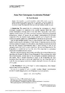
VI. Fig. 9. Density and temperature for iron plasma after 1.2 ns. (a) Electron temperature. (b) Density.

TSA 1976 1230 795

Hybrid 1415 951 590

CONCLUSIÓN

Two methods, namely, DSA and TSA, have been studied and compared. DSA has been shown to have, in general, a better performance than TSA, logical consequence of the fact that a diffusion equation is, in general, much easier to solve than a discrete-ordinate one. DSA has shown this advantage specially in cases with high valué of £ (when acceleration is more needed), high Sn order, and small refinement. However, TSA has shown a good performance for low Sn and high refinement problems. In the light of the results presented, we conclude that TSA can be a good candidate to be used in the resolution of the finer levéis in an AMR scheme.

AMR refinement levéis

APPENDIX Fig. 10. Relative acceleration TSA versus DSA for (triangles) SQ, (squares) Sio, and (diamonds) S14.

To evalúate the performance of the methods, we have chosen an iron laser-created plasma inspired in [18]. It consists in a 1-ns Gaussian láser pulse (A = 800 nm, I = 1.25 x 10 11 W/cm2, and FWHM = 500 /im) over a 100-/im iron slab. For the simulation, we will use a 100 x 100 coarse mesh with two refinement levéis with a refinement ratio of two in a 1.2 x 0.4 mm domain. The time step employed has been Ai = 10 ps. The solvers used to solve the transport and diffusion equations are the same with those in the preceding section. The temperature and density results obtained for a twoAMR-level simulation can be seen in Fig. 9. In Fig. 10, the relative acceleration for different refinement levéis and Sn orders is shown, where it can be observed, as said previously, that the performance of TSA improves when the Sn order is decreased. It should be noted that adding new refinement levéis makes the TSA have a better relative acceleration versus DSA. The reason is the better performance of TSA when the meshes have a bigger refinement, such as those presented in the finest levéis of the resolution. Finally, we have mixed both methods in an AMR simulation. The DSA has been used just to solve the coarse mesh of level 0 and TSA for the rest of the fine meshes (levéis 1 and 2). We have simulated the iron plasma case for different Sn orders with two AMR levéis. The resulting execution times for 1 ns (100 time steps) for this hybrid method in comparison with those obtained just using TSA and DSA are shown in Table IV. From the results, it can be inferred that using both methods is a very effective solution, showing an execution time much smaller than the simulations using TSA or DSA separately. The reason for that is that using DSA in coarse meshes and TSA in fine ones takes the advantages of the properties of both methods.

FOURIER ANALYSIS OF THE M E T H O D S

A) SI Method: The Fourier analysis of the iterative methods will be carried out for a stationary 2-D case, in discrete ordinales, using diamond differencing as a spatial discretization and a backward Euler time differencing in a Cartesian homogeneous mesh. Under these conditions, (6) can be written as follows in each discrete-ordinate direction m with cosines ¡im and rjm and using a level symmetric quadrature: Mm

Ax

l

fjl+1/2 m,i-+ 1 / 2 , J

\>Vm(- •z+1/2 /\y X±m,i,j+l/2

_ T / + 1/2 1

m,i-

i-z+1/2 ± m,i,j-l/2

TZ+1/2_

a

t, i">31m,i,j

'-XijVij^ij^ij

+

Si¿

(18)

where, for simplicity, we have suppressed the g multigroup subscript and normalized the sum of the quadrature weights to the unity. The following expressions must be fulfilled, according to our assumptions: 1 2

7-/+1/2 m,i,j

r/+l/2

m,i+l/2,j

+ ím , ¿ - l / 2 , j

•1+1/2

(19)

1+1/2

(20)

"T"

1

(ji+1/2 2 V m,¿,j+l/2

TI+1/2

m,i,j

+ /;m,i,j-l/2

TV j-Z+1/2 WmI„ m,i,j

¿+1/2 ^ i,3

(21)

771=1

:0'+1/2.

^+1

(22)

To do the Fourier analysis, the variables of the equation are expressed as a Fourier series, obtaining x \A ) i,3

zU)lei°t(\xXi+\yyj)

(23)

x

ttVh*)

(24)

m,i,j

¿~

pivt(\xxi+1/2+\yyj)

(25) (26)

4>\

+l/2

(x)

l

=Lü Be

i,7t{Kx +x v

' «^

(27)

where A^ and Xy are the Fourier modes of the series. Substituting these expressions in (19)-(22), the following equations are obtained:

,¡j, m . fatAxXx\ r^tii 2 i- —— sin . Ax

V

1

r]m .

¡+1 m,i,j

(28) —

(29)

(TtAyXy

= (1 - P)r)XVtFlf

+ VX*t ( V - + V 2 - < , • ) (37)

where Jm,i,j

2 [J"i,i+l/2,j

"•" Jm,i-l/2,j)

*A°)

(30) fl+1

I (fl + 1

=

*=E

, fl + 1

o \Jm,i,j+l/2~

Jm,i,j

N

(31)

\

/am y

•'m,,i,j-l/2j

N

^ ^ Er ^i1 + (/í Ax + m

r¡mKy)2

A,,

2

f

(TtAa;

o"tAj/

atAxXa

with Nlo as the number of directions used to solve the loworder transport equation in TSA and wm as its corresponding weights. By using the following Fourier series:

(32) fm,lj(x)

(33)

tan

=wlamei1+1/2

~ 1).

(35)

The most important aspect in dealing with this equation is the discretization of the spatial derivatives. It has been shown that a discretization inconsistent with the high-order equation can lead to a slow convergence of the method [14]. In the case of a discrete-ordinate transport equation with diamond difference, a consistent scheme is the four-step method, algebraically equivalent to the source correction proposed by Alcouffe [14] and used in PARTISN. Using this discretization, the iteration eigenvalue of the method is [13]

and substituting in (37)-(40) - r~in 2 i-—

Ax

(atAxX sm ,

V

+ atam

* 7 m + 2%— sin (

2

)

^DSA — Wsi +

2

(A x +A y ) + 3 ( l - 0 '

(36)

C) TSA Method: Similar to what has been presented with TSA, to develop the Fourier analysis of TSA, the result of SI can be used, as this is the flrst step of the method. The

Ay

= (1 - fí)r]xatr

+ r]Xat(B

V

2

—y- ) S,

- 1)

atAxXx am = 7m eos

(TtAyXy

(47)

ttm = Sm COS

r = 2_,

(45) (46)

2

w

mam-

m=l

(48)

After some calculation efforts, we obtain

r=

Di(wsi-l) l-Di{l-p)

(49)

where Di is Nlc

3£(^si - 1)

(40)

m=l

where

A,

>

Nlc

Fl+l = V w fl+1

After some algebra simplifleation, the iteration eigenvalue •ujSi can be expressed

^si

,¡+l \ Jm,i-l/2,j)

V 2

fatAxX;,

am = Sm eos

_

fatAy\y

+ 0"í«m = XVa t

7m eos I

Mm / , ¡ + l ¿±x \Jm,i+l/2,j

7 m + 2»-—sin '

Ay

2

analysis of the method would continué by examining the second transport equation, which we will suppose is fully converged

£>i =