National Biological Service, Georgia Cooperative Fish and Wildlife Research Unit*. Daniel B. Warnell School of Forest Resources, University of Georgia, Athens.
North American Journal of Fisheries Management 15:940-955. 1995 © Copyright by the American Fisheries Society 1995
Comparison of Catch Rate, Length Distribution, and Precision of Six Gears Used to Sample Reservoir Shad Populations MICHAEL J. VAN DEN AVYLE National Biological Service, Georgia Cooperative Fish and Wildlife Research Unit* Daniel B. Warnell School of Forest Resources, University of Georgia, Athens. Georgia 30602 USA
JEFF BOXRUCKER Oklahoma Department of Wildlife Conservation 500 East Constellation. Norman. Oklahoma 73972 USA PAUL MlCHALETZ Missouri Department of Conservation 1110 South College Avenue. Columbia. Missouri 65201, USA
BRUCE VONDRACEK National Biological Service. Minnesota Cooperative Fish and Wildlife Research Unit2 University of Minnesota. 1980 Folwell Avenue. St. Paul, Minnesota 55108. USA
GENE R. PLOSKEY U.S. Army Engineers Waterwavs Experiment Station 3909 Halls Ferry Road (CEWES-ESQ). Vicksburg. Mississippi 39180. USA Abstract.—Hydroacoustics, trawling, gillnetting, electrofishing. shoreline seining, and cove rotenoning were used concurrently in August 1991 at Lake Texoma, Texas-Oklahoma, to compare sampling efficiency for gizzard shad Dorosoma cepedianum and thread fin shad D. petenense. A simple randomsampling design was used at nearshore and offshore stations in each of three 400-2,000-ha sites in the reservoir. Most gears provided similar evidence of spatial patterns of shad abundance among sites, but length distributions and sampling precision varied among methods. At offshore transects, catch-perunit-effort (CPUE) data for hydroacouslics, trawling, and gillnetting were positively correlated (r = 0.45-0.80; P < 0.05) when data from all sites were combined. Gears differed in proportions of small (age-0) shad versus larger (age-1 and older) fish. Gears that collected mainly age-0 shad were trawls, surface-set gill nets, and seine, whereas catches of age-1 and older shad were greater with bottom-set gill nets, electrofishing, and rotenone. Sampling precision, as measured by the coefficient of variation (CVx = SD/mean) among replicate samples for each species and site, ranged from 0.2 to 0.7 for hydroacoustics, surface-set gill nets (both species), trawl (threadfin shad), and rotenone (gizzard shad). Poorer precision was obtained with the seine (1.0-3.2, both species), electrofishing (0.7-1.8, both species), bottom-set gill nets (0.4-1.7. both species), trawl (1.0-1.5. gizzard shad), and rotenone (0.8, threadfin shad). We quantified relative gear efficiency by calculating the number of replicate samples needed to estimate median CPUE within 25% of the true median at 95% probability and multiplying this by the hours of labor required to obtain one replicate. Most labor estimates for hydroacoustics, trawling, and surface-set gill nets were less than 120 h (one week of work for three people); requirements were usually much greater for rotenone (1,524-5,384 h). seining (114-954 h), electrofishing (171-973 h), and bottom-set gill nets (53-418 h). The number of replicate samples needed to attain the desired precision criteria was 14-25 for hydroacoustics. 9-79 for trawling, and 5-55 for surface-set gill nets.
We evaluated the relative effectiveness of six commonly used sampling gears for quantifying ____ .. . . , ., . , 1• ^ t t . . . . . The Unit is jointly sponsored by theKINational 0Biological Service, the Georgia Department of Natural Resources, the University of Georgia, and the Wildlife Management Institute.
abundance and length distributions of gizzard shad Dorosoma cepedianum and threadfin shad D. petenense in reservoirs. Gears included trawls, hydroacoustics, gill nets, electrofishing,° cove rotenone, ° and semes. Shad are important components of reservoir ecosystems, where they often are the major
tute.
regulate overwinter survival of important predators
2 The Unit is jointly sponsored by the National Biological prey of piscjvorous fishes (Noble 1981). The abunScrvice, t h e Minnesota Department o f Natural Resources, t h dance e ' and . ,slze . r i _ j • • University of Minnesota, and the Wildlife Management InstiStructure of shad populations can
940
GEARS COMPARED FOR SAMPLING SHAD
like largemouth bass Micropterus salmoides (Adams and DeAngelis 1987), and shad also may regulate survival of young sport fishes via competition for zooplankton (DeVries and Stein 1992; Dettmers and Stein 1992). Shad have been widely stocked in reservoirs in managers' attempts to increase prey availability (DeVries et al. 1991). Despite the importance of shad to reservoir fisheries, little research has been done on the comparative efficiency of commonly used sampling gears. Hayne et al. (1967) and Aggus et al. (1980) evaluated the use of rotenone to sample coves, and Johnson et al. (1988) compared density estimates from a Tucker trawl, seine, and shoreline rotenone quadrats. Michaletz (in press) compared catch data for gizzard shad collected by electrofishing and gill netting. Midwater trawls, which were first used for sampling reservoir fishes in the 1960s (Houser and Dunn 1967), provided more precise estimates of shad abundance in a North Carolina reservoir than those obtained with cove rotenone sampling (Siler 1986). Knowledge of sampling biases, precision, and labor costs associated with different gears is needed to optimize shad sampling programs and improve fisheries management decisions. In this study, we used multiple gears concurrently to evaluate differences in size selectivity, compare sampling precision and cost efficiency, and determine if catch rates were correlated among methods. Our analyses combine selected data obtained in several more specific gear evaluations conducted simultaneously at Lake Texoma, Texas-Oklahoma, in August 1991 (Boxruckeret al. 1995, this issue). In cases in which several versions of one gear type were originally compared, we selected the version recommended as most effective by authors of copublished papers in this issue (Michaletz et al., trawls; Degan and Wilson, hydroacoustics; Van Den Avyle et al., gill nets; DeVries et al., electrofishing).
Methods Study Area Sampling was conducted on 12-15 August 1991 in two large embayments and the Central Pool of 35,600-ha Lake Texoma, Texas-Oklahoma (Figure 1). These sites represented the range of morphometric and limnological conditions present in the lake and were expected to have different shad densities (Boxrucker et al. 1995). The larger embayment, Big Mineral (2,000 ha), had a mean depth of 5 m and substrate of mud and sand. Little Mineral embayment (400 ha) had a mean depth of 13
941
m and substrate of gravel, rock, and boulders. The 2,000-ha portion of the Central Pool that was sampled had a mean depth of 20 m and sandy shoreline substrate; this site included the deep (25-30 m), inundated channel of the Red River. During summer, the lake is vertically stratified, with oxygen depletion in the hypolimnion (Hubbs et al. 1976). During our study, surface water temperature was 27-29°C, and dissolved oxygen concentration was 6-8 mg/L; dissolved oxygen was less than 2.0 mg/ L at depths greater than 10 m (Boxrucker et al. 1995). Conductivity at the surface ranged from 990 u,S/cm in Little Mineral embayment to 1,390 u,S/ cm at Big Mineral. Sampling Design Gear comparisons were based on simple random sampling within offshore and nearshore strata of each study site. Results were used to estimate shad length-frequency distributions, variation in abundance among sites, and variance of catch-per-uniteffort (CPUE) data. Additionally, we determined the amount of effort (person-hours) required to use each gear type and process the collected fish. These data were used to calculate sample sizes and labor requirements needed to attain predetermined standards for precision of CPUE estimates. Data were obtained either for all species of fish or for shad and Morone spp., but our analyses are restricted to shad. Results for juvenile Morone spp. were reported by Neumann et al. (1995, this issue). At each study site, contour maps were used to identify all possible 0.25-km2 offshore sampling stations in areas 7 m or more deep, and 20 stations were selected at random to be sampled with trawls, hydroacoustics, and surface-set gill nets (Figure 1). Stations were marked with buoys, and gill nets were set before dusk. After dark, we collected data first with hydroacoustic equipment and then with trawls by sampling transects parallel to each gill net. This allowed estimation of correlation coefficients for CPUE among the three gears. Equipment failures resulted in sampling of only 15 offshore stations by gill net in Little Mineral embayment and 18 stations by hydroacoustics in Big Mineral embayment. Nearshore sampling stations were established as 500-m transects along the shoreline (Figure 1). From all possible transects at each site, 20 were randomly selected for sampling with electrofishing (DeVries et al. 1995). Electrofishing equipment did not operate properly at Big Mineral embayment
(the first night of sampling). We established nearshore gill-netting stations at each site by randomly
942
VAN DEN AVYLE ET AL.
FIGURK 1.—Study sites used to compare shad sampling gears at Lake Texoma, Texas-Oklahoma. Sampling stations are coded as open circles (offshore transects for hydroacoustics, trawls, and surface-set gill nets), solid triangles (nearshore stations for surface- and bottom-set gill nets), solid circles (shoreline electro fish ing transects), S (shoreline seining stations), and R (coves sampled with rotenone). The dashed line indicates the 7-m depth contour.
selecting a subset of five electrofishing transects and moving away from the shoreline until a depth of 6-8 m was reached. Two nets were set at each station, one at the surface and one on the bottom. Shoreline transects were also sampled with a seine during daytime; 10 stations were randomly selected at each site. By chance, 11 of the 30 transects selected for seining coincided with those selected for electrofishing. We sampled one small cove in each study site by applying rotenone (1 mg/L) and retrieving fish for 2 d. A block net was installed across the mouth of each cove before application of rotenone. Surface area of the coves was 0.44-0.73 ha, and mean depth was 1.5-2.0 m. Gear Descriptions
Gill /n/.v.-Van Den Avyle el al. (1995) compared the efficiency of horizontal and vertical gill nets for sampling shad and found that horizontal nets
provided more precise results. Thus, our analyses are restricted to horizontal nets. Each net was 2.4 m tall and 76.5 m long, and each included 10 monoftlament panels (each 7.6 m long and hung on a one-half basis) with mesh sizes (bar measure, mm) of 10, 12, 19, 25, 38, 51, 64, 76, 89, and 102. Twine sizes were number 69 (0.28 mm) for the 10-38-mm meshes, number 139 (0.40 mm) for the 51-76-mm meshes, and number 177 (0.47 mm) for the 89-102-mm meshes. Nets were set before dusk (1700-2100 hours) and retrieved the following morning (0700-1200 hours), with an average set duration of 15.7 h (SD = 2.2 h). Mesh size, species, and total length (mm) were recorded for all fish. When a large number of fish were collected, the sample was placed on ice and returned to a laboratory for processing. Subsamples of 100 individuals of each species
were used to estimate length-frequency distributions for each mesh size of each net. The CPUE
GEARS COMPARED FOR SAMPLING SHAD
data were summari/ed as number per net; results were not adjusted for set duration because CPUE was not correlated with soak time (Van Den Avyle et al. 1995). We determined processing time for each net as the person-hours required for retrieval and to remove, identify, measure, and record the data for all fish. We also determined the amount of time required to set and lift the nets. Crew size was three people per boat. Time required for lab work was added to the processing time just described. Trawls.—Michaletz et al. (1995) concluded that paired l-m 2 frame trawls and a 1.67-m2 Tucker trawl provided the most similar estimates of shad density obtained in four types of trawls used to sample juvenile shad in Lake Texoma. Density estimates were most precise for the frame trawl; consequently, we used the results from only frame trawls. The trawls (6.4-mm mesh) were towed at night at a speed of 1.6 m/s in a stepwise oblique pattern and sampled 1 min at each of four depths (in sequence): 0.5, 2.5,4.5, and 6.5 m. Deployment and retrieval of the nets required about 0.75 min, making the total sampling time about 4.75 min. A flowmeter in the mouth of each net measured sample volume, which averaged 9 1 0 m 3 for the two nets combined. For each transect, collections were combined for the two nets and returned to the laboratory for identification, counting, and measuring. The CPUE was expressed as the number of fish per 1,000 m3. A crew of three people was used for trawling. Sampling effort was quantified as the amount of time required to collect all samples plus the time of travel to and from the launch site. The amount of time needed to process the fish collected was recorded separately for each transect. Hydroacvustics.—Degan and Wilson (1995) recommended using a hydroacoustic frequency of 120 or 200 kH/ at night for estimating abundance of pelagic fishes in Lake Texoma. We used data reported by Degan and Wilson for 200 kHz because it provided greater estimates of fish abundance. The system consisted of a dual-beam transducer (6° x 15° nominal, circular), a scientificgrade echosounder, and a digital data recorder. The transducer was mounted on a fin at the bow of a boat (depth, 0.75 m) and pushed at 1.5 m/s for 5 min at each sampling transect. The system was adjusted to collect data for fish longer than 25-30 mm total length at depths from about 2 m below the surface to I m above the bottom. Results were expressed as the average number of fish per 1,000 m3 for a depth range of 2-7 m. This facilitated
943
comparisons with trawls, which sampled depths of 0-7 m. Fish length-frequency distributions at each site were estimated with a regression model that predicted fish lengths from the acoustic strength of individually tracked targets (Degan and Wilson 1995). The model was calibrated with lengths of thread fin shad collected in trawls. A crew of three people was used to acquire hydroacoustic data. We recorded the amount of time required for field calibration, sampling, and travel between launch sites and transects. The time required to convert field data into density estimates and length-frequency distributions was also determined. Electrofishing.—DeVries et al. (1995) compared electrofishing samples for shad in Lake Texoma with two fish-retrieval methods: dipnetters and a less labor-intensive push net. The use of dipnetlers to retrieve fish is more conventional, and we include only these data in our evaluation. Results can be extrapolated to the push-net method with data presented by DeVries et al. Electrofishing was conducted after dark with 15 min of effort (pedal time) at each transect, and data were recorded as number per hour. Fishes other than shad and Morone spp. were not collected. All boats used 5,000W generators and Smith-Root GPP 5.0 electrofishers set to operate at 10-12 A and 300 V. Collected fish were stored on ice and processed after all transects were sampled. Crew size for electrofishing was three people, including a boat operator and two netters. Sampling effort and fish processing time were measured as for trawling. Seine.—Samples were collected during the day (preceding nighttime sampling by other gears) with a 15.4-m X 1.8-m bag seine with 6-mm mesh. At each transect, one seine haul was made covering about 200 m2. Fish were immediately processed, and results were recorded as number per haul. Time required to travel among transects, collect samples, and process fish was recorded for each sample. Crew size was three people. Rotenone.—Coves were sampled by personnel of the Texas Parks and Wildlife Department and Oklahoma Department of Wildlife Conservation. Methods followed those described by Davies and Shelton (1983). All recovered fish were counted and weighed by species and inch-group (25.4-mm) categories. To obtain length-frequency data comparable to those of other gears, we measured subsamples of each inch-group of thread fin shad and gizzard shad to the nearest millimeter total length. Results were expanded within inch-groups and
944
VAN DEN AVYLE ET AL.
summed within each cove according to millimetergroups. Abundance was calculated as number per hectare. Crew size for cove sampling was 3-4 people for installing and removing the block net, 3-4 for applying rotenone, 8-14 for retrieving, sorting, measuring, and counting all species of fish by inchgroups, and 2 for measuring subsamples of shad for millimeter-groups. We recorded the total number of person-hours required for each category of work at each cove. Data Analyses Length distribution.—We used Smirnov tests for pairwise comparisons of shad length distributions between gears (Conover 1971). Data were sorted by species and summarized for 10-mm (midpoint)
pare sites. For a given gear, we converted each CPUE observation to standard measure by subtracting its overall mean value (sites pooled) and dividing by the standard deviation. The result is a unitless measure of the number of standard deviations from the overall mean. Average values of the standardized data were calculated for each site, and spatial patterns were compared among gears. Sampling precision and required sample size. — We compared precision of CPUE estimates among gears by calculating the sample coefficient of variation, CVX (= SD/mean, where X = CPUE). Gears that yield high values of CV^ provide relatively imprecise data and require greater sampling effort than gears with low CV*. Estimates were computed separately for each site to illustrate variation that might be encountered in other reservoirs or at
length-groups; sites were tested separately because
other times. For rotenone, CV# was calculated
distributions varied significantly (P < 0.05) among among sites because there was no replication withsites for most gears. Comparisons were made sep- in sites. arately by species and for fish that were either age We compared sampling efficiency of the various 0 or age 1 and older because of variation among gears by calculating the amount of labor (L,y*) gears in catching fish older than age 0. Delimiting needed to achieve a specified level of precision of sizes were 150 mm for gizzard shad and 100 mm CPUE: for threadfin shad (Oklahoma Department of Wildlife Conservation, unpublished data). Hydroacoustic data were not compared statistically with Njjk = number of replicates needed; those of other gears because target-strength disQ- = person-hours of labor required per replitributions had been adjusted to coincide with the cate; length distribution of threadfin shad in trawls (Dei = species; gan and Wilson 1995). Hence, comparisons inj = sampling site; volving hydroacoustic data would be equivalent to k = gear type. those of trawl data for threadfin shad. Because We estimated Q by averaging for all sites the efSmirnov tests are highly sensitive to small differfort needed to use each gear and process the fish. ences between length distributions when sample Our goal for precision was to estimate CPUE sizes are large, we used P = 0.01 to judge statiswithin 25% of the true median at a 95% probability tical significance. Tests were not performed when level. This precision corresponds to standards essample size was less than 30 fish. tablished for "management studies" by Robson Spatial patterns.—To determine if gears reand Regier ( 1 964) in their determination of sample vealed similar spatial patterns of abundance, we sizes required for Petersen mark-recapture popuestimated correlation coefficients between CPUE lation estimates. We calculated for gears used at the same transects and compared average CPUE of each gear among sites. CorreNijk = (2? *2)/[log,(RE + 1)|2; lation analyses were conducted for (1) hydroacousZ = 1.96, the ordinate of the normal curve at tics, trawls, and gill nets at offshore transects; (2) the 95% confidence level; surface- and bottom-set gill nets at nearshore trans2 = variance of transformed data [log^CPUE sects; and (3) seining and electrofishing at shore+ »; line transects. Density estimates made with hyRE = 0.25, our target for relative error about the droacoustics were regressed on those made with median CPUE (Gilbert 1987). trawls to evaluate correspondence. Because both gears measured density as number per 1,000 nv\ This equation simplifies to N^ = 77 s2 for the the regression line was expected to have slope = specified values of Z and RE. This approach ap1 and intercept = 0. propriately assumes that CPUE data were lognorWe standardized average CPUE values to com- mally distributed and uses variance properties of
GEARS COMPARED FOR SAMPLING SHAD
TABLE 1 . — Number of fish collected in sampling gears used at three sites in Lake Texoma . August 1991. Gear and site
Gi//ard Thread- Other shad tin shad species
Total
Hydroacousiics0 Central Pool Little Mineral Big Mineral All .sites Trawl Central Pool Little Mineral Big Mineral All sites Gill net (offshore, surface) Central Pool Little Mineral Big Mineral All sites Gill net (nearshore, surface) Central Pool Little Mineral Big Mineral All sites Gill net (nearshorc. bottom) Central Pool Little Mineral Big Mineral All sites Electrofishingh Central Pool Little Mineral All sites Seine Central Pool Little Mineral Big Mineral All sites Rotenone Central Pool Little Mineral Big Mineral All sites
1.270 11.905 8.189 21,364 1.892 2.705 7.275 11.872 1.635 3.167 9.630 14.432 4,797 17.777 25,094 47,668
Gears and sites combined (excluding hydroacou sties)
18,226 76,346 28,103 122.765
3.506 3,178 928 7.612
0 21 385 406
979 3.538 9,773
945
TABLE 2. — Between-gear comparisons of length distributions for gizzard shad and thread fin shad collected in various gears at three sites in Lake Texoma, August 1991. Results for age-0 fish are presented in the upper right portion of each matrix, and fish older than age 0 (age 1 + ) in the lower left. Each entry consists of three symbols indicating results of separate Smirnov tests for (respectively from left to right) samples in the Central Pool. Little Mineral embayment, and Big Mineral embayment. Symbols are: * significant at P = 0.0 1; n = not significant; and • = at least one gear with fewer than 30 fish. Abbreviations are: OS, offshore, surface; NS. nearshore surface; NB, nearshore bottom.
I*T,ZV\J
Id *)W\
13 12 26 51
992 3,571 10.184 14.747
77 1.850 899 955 6.965 26.309 7.941 29,114
271 403 616 1.290
2.198 2.257 33.890 38.345
177 644 692 1.513
956 2,850 1.386 5.192
74
1.207 3.628 2,204 7.039
Gill net, NS Gill net. NB Trawl Electrofishing Seine Rotenone
94 138 279 511
189 253 1.086 1,528
287 892
537 742 1.652 2,931
Threadfln shad: age 1 + (below diagonal), age 0 (above diagonal) Gill net, OS n*n *n* *** **• •** ***
1,696 347 2.043
2.469 1.017 3.486
37 217 254
4,202 1.581 5.783
133 357 525 1,015
19 1,382 3,558 4.959
45 12 131 188
197 1.751 4,214 6.162
Gill net. NS Gill net. NB Trawl Electrofishing Seine Rotenone
134 126 334 254
351
a
Values shown arc numbers of individually identified targets within a depth range of 2-7 m. h Species other than shad and Morone spp. were not collected; data were not obtained at Big Mineral embayment.
log-transformed data for determining sample sizes accordingly (Gilbert 1987).
Results The total number of fish collected in all gears was 122,675, including 18,226 gizzard shad, 76,346 threadfin shad, and 28,103 specimens of other species (Table 1). The proportion of nonshad fishes ranged from 0.3% in trawls to 52.6% in cove rotenone samples; a low proportion for electrofishing (4.4%) reflected active avoidance by dipnetters of species other than shad or Morone spp.
Gear
OS
Gill net
_FWtnv-
NS
NB Trawl fishing Seine none
Ron..
Gizzard shad: age 1+ (below diagonal), age 0 (above diagonal) Gill net, OS nnn ••* ••* **• *** 0n* •** •»+ •*• •** •**
••* ••* **• **n ••* ••• »+• ••• »+• **• **• ••• •** •** ••• •*• *n* *** ••• **•
*** ••* ••* **•
n** n** ••* ••* **• •nn ***
n** *** *** »*• •** nn* nn* *** n** •** »+•••••»• *•• •** •*• •*• •*• ••• •*• ••• ••• +++ ••• •++ *•• *•• *•• ••• ••+ +++
*** *** *" **• •**
(DeVries et al. 1995). Threadfin shad were more numerous than gizzard shad in all gears, but composition varied among gears (Table 1). The ratio of thread fin shad to gizzard shad was about 2 for electrofishing, 3-4 for gill nets and rotenone, 5 for seining, and 35 for trawling. Length Distribution Length distributions of both gizzard shad and threadfin shad differed significantly among gears in most cases in which sample sizes were adequate for statistical analysis (Table 2). Length distribution of age-0 gizzard shad differed significantly (P < 0.01) among most gears, but relations among gears differed with site. At Central Pool, median length was 50 mm for seine samples, 80 mm for electrofishing, and 100 mm for gill nets and rotenone (Figure 2). At Little Mineral embayment, median length was 90-100 mm in all gears except the trawl, which collected smaller fish (median = 70 mm). At Big Mineral, median length was 90100 mm in trawls and gill nets and 110 mm in
electrofishing, seine, and rotenone samples. Sample sizes in gill nets set near shore on the bottom
946
VAN DEN AVYLB ET AL.
50
Central Pool N =0
40
Little Mineral Trawl N=21
Big Mineral N-385
30 20 100
Gillnet
40-
N=8M
(offshore, surface)
30 20 10 -
t hi 40-
.,.».n*.
30 0- 20^ 10 0 70 6050 40 30 20 • 100 70 • 605040302010 0 70
Central Pool
Little Mineral Trawl N=3SM
N = 979
N = 1850
Big Mineral
A a Gillnet
N=795S
Gillnet
N=285
Gillnet
N=253
= 9773
N = 26309
(offshore, surface)
= 956
(nearshore, surface)
N=189
1386
°
1086
(nearshore, bottom)
LL
2469.
= 38
Electrofishing 1017
19
N = 11905.
:
60 504030 20 10 : 0 50
100
150
0
Seine
N = 1382
Rotenone
N=27M
«ii 50
100
150
0
^
JL .illi 50
100
3558
N = 3167
150
200
Total Length (mm) FIGURE 3.—Length distribution of Ihreadfin shad collected at three sites in Lake Texoma, August 1991.
GEARS COMPARED FOR SAMPLING SHAD
949
TABLE 3.—Correlation between catch rates of gizzard shad, threadtin shad, and all shad combined collected with various gears at three sites and for sites combined at Lake Texoma, August 1991. Coefficients followed by an asterisk were significantly different from 0.0 at P = 0.05; W is the number of pairs of observations.
sites and species, but no consistent patterns were evident (Table 5).
labor requirements varied considerably among
estimating CPUE within 25% of the true median
Discussion None of the six gears we evaluated was clearly superior for sampling reservoir shad populations. Correlation coefficients for Gears differed according to sizes of shad collected, Threadtin relative proportions of shad and other fishes colGi//ard shad shad Site All shad lected, sampling precision, and labor required to Hydroacoustics versus trawl obtain CPUE estimates at a specified precision. Central Pool 20 nca 0.36 0.36 Consequently, the choice of sampling method de0.62* Little Mineral 20 0.52* 0.52* pends on the target species and sizes of fish to be 0.06 18 -0.56* Big Mineral -0.53* sampled as well as the budget for a given study. 58 0.44* Sites combined 0.36* 0.45* For example, at offshore sites, hydroacoustic gear Hydroacoustics versus gill net (offshore, surface) Central Pool 20 -0.03 0.02 0,01required only 14-25 h of labor to obtain precise Little Mineral 15 -O.I I 0.19 0.18 data, but the method was effective only for small Big Mineral 20 -0.07 -0.19 -0.18 fish ( small to estimate coefficients for separate sites. sampling tool can be evaluated according to the amount of labor required to obtain acceptably precise CPUE estimates. We assume that few manto each study site (to deploy nets and to retrieve agement agencies would allocate more than 120 h them) and required extended effort in the lab to of labor to obtain one estimate of shad abundance. process the numerous fish collected, used about This is equivalent to 1 week of work for a crew 4.4 person-hours per replicate. of three people. Given this assumption and the The amount of labor needed to estimate CPUE sampling variance at Lake Texoma, sampling does within 25% of the true median with 95% proba- not appear economical with rotenone (1,524-5,384 bility was least for hydroacoustics and greatest for h), seining (114-954 h), electrofishing (171-973 rotenone (Table 5). The low requirements for hy- h), or bottom-set gill nets (53-418 h). The majority droacoustics, 14-25 person-hours, are attributable of labor estimates were less than 120 h for hydroto its relatively good precision, small required acoustics, trawling, and surface-set gill nets (Table sample size, and minimal labor per replicate (Table 5). Based on averages for both shad species at three 4). Rotenone, however, has relatively poor preci- sample sites at Lake Texoma, the approximate sion, high required sample size, and per-sample number of replicate samples needed to attain prelabor that greatly exceeds that of the other gears, cision criteria of "management studies" (sensu leading to labor requirements of 1,524 h for giz- Robson and Regier 1964) would be 19 for hydrozard shad and 5,384 h for thread fin shad. acoustics, 45 for trawling, 26 for surface-set gill Other gears with relatively high labor require- nets at offshore stations, and 16 for surface-set gill ments included the seine (114-954 h), electron'sh- nets at nearshore stations. ing (171-973 h), and bottom-set gill nets at nearRequired sample sizes and resultant labor costs shore stations (53-801 h; Table 5). Trawls and sur- are highly dependent on desired goals for preciface-set gill nets were estimated to require 15-242 sion. We chose the criteria of Robson and Regier h. For each gear except hydroacoustics, estimated (1964) for "management studies" with the goal of
950
VAN DEN AVYLE ET AL. 100
GizzardShad r»0.58;N«55 P < 0.0001
80-
A A
40-
20AA A
OH>
250
500
1000
750
Gillnet, offshore (fish/net)
1UUU -
B
Threadfin Shad r«0.80;N>55
A
p < 0.0001
A
^r800-
A A
5
A
§600-
A