Comparison of Common Homology Modeling Algorithms: Application of User-Defined Alignments. Michael A. Dolan , James W. Noah , and Darrell Hurt. Abstract.
Chapter 18 Comparison of Common Homology Modeling Algorithms: Application of User-Defined Alignments Michael A. Dolan, James W. Noah, and Darrell Hurt Abstract The number of known three-dimensional protein sequences is orders of magnitude higher than the number of known protein structures. This is a result of an increase in large-scale genomic sequencing projects, the inability of proteins to crystallize or crystals to diffract well, or a simple lack of resources. An alternative is to use one of a variety of available homology modeling programs to produce a computational model of a protein. Protein models are produced using information from known protein structures found to be similar. Here, we compare the ability of a number of popular homology modeling programs to produce quality models from user-defined target–template sequence alignments over a range of circumstances including low sequence identity, variable sequence length, and when interfaced with a protein or small molecule. Programs evaluated include Prime, SWISS-MODEL, MOE, MODELLER, ROSETTA, Composer, ORCHESTRAR, and I-TASSER. Proteins to be modeled were chosen to test a range of sequence identities, sequence lengths, and protein motifs and all are of scientific importance. These include HIV-1 protease, kinases, dihydrofolate reductase, a viral capsid protein, and factor Xa among others. For the most part, the programs produce results that are similar. For example, all programs are able to produce reasonable models when sequence identities are >30% and all programs have difficulties producing complete models when sequence identities are lower. However, certain programs fare slightly better than others in certain situations and we attempt to provide insight on this topic. Key words: Homology modeling, Comparative modeling, Sequence alignments, Protein modeling software, Loop modeling
1. Introduction Obtaining the three-dimensional structure of a protein often proves to be challenging, employing techniques such as X-ray crystallography and NMR, sometimes taking years to yield results. Frequently, the structure of a protein cannot be determined by X-ray crystallography because it cannot be crystallized or if coaxed into crystallizing, will not diffract well. Similarly, a protein may be Andrew J.W. Orry and Ruben Abagyan (eds.), Homology Modeling: Methods and Protocols, Methods in Molecular Biology, vol. 857, DOI 10.1007/978-1-61779-588-6_18, © Springer Science+Business Media, LLC 2012
399
400
M.A. Dolan et al.
unsuitable for NMR experiments due to relatively large size or because of aggregation. One example is that of the membranebound G-protein-coupled receptor (GPCR) family of proteins where crystal structures traditionally have been difficult to obtain (1, 2), although recent efforts resulting in determination of the human β2-adrenergic GPCR structure should be noted (3–5). Experimental difficulties coupled with the availability of approximately five million protein sequences (6) and limited amount of resources to experimentally derive three-dimensional structures make an alternative method of structure determination desirable. Creating a three-dimensional protein model based on information from similar or “homologous” proteins whose structures are known is a faster way of gaining structural insight compared to experimental methods and is often the only way to obtain a threedimensional view of a protein. The classic paradigm of constructing a homology model is to first find proteins that are homologous to a query or “target” sequence and align them according to common sequence and structural features. The next step is to construct a backbone model consisting of regions that are structurally conserved across the homologs followed by building regions that vary structurally, often comprising loops, insertions, or deletions (“gaps”) relative to homologous regions. The final step is to add side chains to the backbone followed by a minimization or molecular dynamics protocol to lower the overall energy of the structure by correcting any bad geometries or steric problems. Over several decades, a number of homology modeling packages have been developed that rely on knowledge-based methods, ab initio methods or a combination of the two to produce a protein model. Knowledge-based programs such as SWISS-MODEL (7), PROFIT (8), ICM (9), and ROSETTA (10) use information from known structures, often represented as a library of fragments to construct a three-dimensional model from a target sequence. Homology modeling programs such as MODELLER (11) use ab initio methods producing solutions that satisfy a set of spatial rules derived from probability density functions and statistical analysis of a protein structure as a whole. ORCHESTRAR (12–16), Composer (17, 18), GENEMINE/LOOK (19), MOE (20), and Prime (21) use a combination of ab initio and knowledge-based approaches. A difficult question then arises: how does one evaluate the quality of a model? One obtains a different answer depending on the nature of the question asked and the method used for evaluation. For example, if the overall fold of a large protein (~500 residues) is compared by measuring the root-mean-square deviation (RMSD) between the backbone atoms of the model to a solved structure, the resulting value may not be as good as if one compared individual domains in the same way, due to differences in overall domain orientations between the model and the solved structure. In this case, one would better understand model quality
18
Comparison of Common Homology Modeling Algorithms…
401
by comparing the individual model domains to the solved structure domains, and looking at domain orientation separately. The message to the reader is to take comparative results with a grain of salt: look very closely at the methods used to make comparisons and what was compared, whether it is part of or the entire model, which atoms were used in the comparison, what stage of the modeling process is being compared, and the quality of the template to which the model is being compared. A wide variety of protein homology modeling algorithms have participated over the years in the Critical Assessment for Structure Prediction (CASP) (22) where researchers are given a set of sequences that have known, but yet to be released three-dimensional structures. Three-dimensional solutions are submitted, evaluated and compared to the known protein structures, once the contest ends. Like CASP, this study compares the capability of popular homology modeling packages to produce models of proteins whose three-dimensional structures are known with an exception being that each program is provided identical, specific, user-defined alignments as input. Unlike CASP, it attempts to produce models that use only the default settings of the programs and does not include any additional energy refinement procedure at the end of the modeling process. An attempt is made therefore, to assess only the structure building capabilities of each program. Importantly, modeling using multiple homologs was not examined in this study as not all programs evaluated are able to use information from multiple templates across all parts of a model. In order to include a wider variety of programs, we opted to produce homology models based only on a single template. Of note, although other comparisons have been performed (23–25), this is the first study to evaluate ORCHESTRAR, a more recently developed homology modeling package, when compared to a number of different programs. Finally, we make little attempt to gauge the userfriendliness of the software as this can be subjective between researchers, but instead refer the reader to usability information found in other studies (23–25).
2. Materials 2.1. Sequence Selection
A total of 18 protein sequences were chosen that provided a range of sequence lengths and sequence identities as well as a wide variety of protein folds. Sequences range from 46 to 504 residues and have identities to templates of between 17 and 94%. A number of pharmaceutically relevant proteins were examined including several kinases, dihydrofolate reductase (DHFR), HIV-1 protease, and factor Xa, among others. Protein models are often produced with the intent of using the model for peptide or ligand-binding
402
M.A. Dolan et al.
studies or for examining protein–protein interactions. Therefore, we examined in detail those models produced from homologs containing a protein–protein interface, peptide, or small moleculebinding site and determined how well each program reproduced these regions. Specifically, we examined backbone atom and allatom positions within 5 Å of these regions. 2.2. Software
Default settings were used for all software except for those that modeled termini and those that allowed additional minimization of the final model with the exception of SWISS-MODEL where it is not possible to produce models without modeling the termini or minimizing the final structure. For all other programs, an all-atom minimization is not performed, but each program has internal optimization strategies for modeling including those that add and optimize side-chain positions. 1. ORCHESTRAR ORCHESTRAR (distributed by Tripos) is comprised of a group of algorithms including programs to structurally align homologs (Baton) (15, 16), generate conserved region models (CHORAL) (12), find structurally variable regions or “loops” using knowledge-based and ab initio methods (PETRA and FREAD) (14), and add side chains (ANDANTE) (13). 2. Prime Prime (developed and distributed by Schrödinger, LLC) constructs a model using aligned atom positions of homologs. Default settings use the OPLS force field (26, 27) and a surface-generalized Born solvent model (28). Prime constructs model regions not derived from the templates by an ab initio method (29) while side-chain conformations are taken from a rotamer library. In this study, we used default settings with the exception of building terminal tails beyond secondary structure elements and minimizing residues. 3. MOE MOE-Homology (developed by Chemical Computing Group, Inc.) combines the methods of segment-matching procedure (19) and the approach to the modeling of insertion/deletion regions (30). MOE-Homology creates ten models by default using a knowledge-based loop searching method and sidechain rotamer selection method after which an average model is created and then submitted to a user-controlled energy minimization. In our study, the “Best Intermediate” model was chosen using the default settings with the exception of a minimization. 4. SWISS-MODEL Differing from the other modeling methods in the study, SWISS-MODEL (7) is a fully automated comparative protein modeling server (http://swissmodel.expasy.org/). The Alignment
18
Comparison of Common Homology Modeling Algorithms…
403
Mode was used which takes an aligned query–template sequence as input and uses the knowledge-based ProModeII (31) program to produce a model. SWISS-MODEL attempts to produce a complete, minimized model using the Gromos96 force field (32). 5. Composer The Composer program (17, 18) was integrated into SYBYL (distributed by Tripos) prior to version 8.0. The alignment portion of the program was bypassed to preserve the alignment of the input. In default mode, Composer uses structural alignment information from multiple templates to first define structurally conserved regions (SCRs) across all homologs which it then uses to construct a partial model. Any remaining gaps or structurally variable regions (SVRs) between SCRs are modeled using a loop modeling algorithm. When only a single template is used for model construction as in this study, Composer defines an SCR as those regions where no gaps occur between the alignment of the target and template sequences. 6. MODELLER MODELLER uses the “automodel” class to construct a three-dimensional model of the target protein. Model building is implemented by satisfaction of spatial constraints (11). Target/templates were submitted to the program and five models were generated and evaluated. Top models were chosen based on discrete optimized protein energy (DOPE) score (33, 34). 7. Rosetta Homology models were constructed using Rosetta version 3.1 which leverages the loop modeling algorithm within the Rosetta software suite. For each target, 10K models (referred to as “decoys”) were generated using the Biowulf Linux cluster (National Institutes of Health, Bethesda, MD; http://biowulf.nih.gov). The top 1,000 decoys in terms of lowest energy were clustered using an RMSD of 5 Å between decoys. The energies of representative decoys from each cluster were obtained and the representative decoy having the lowest overall energy was taken as the “correct” solution. 8. I-TASSER Sequence alignments were submitted to the I-TASSER server (35) after selecting the option “Specify template with alignment.” This option allows one to specify both the template structure and the target–template sequence alignment. This differs from the default mode where one submits the target sequence only and allows the program to provide templates and sequence alignments.
404
M.A. Dolan et al.
3. Methods 3.1. Sequence Selection
Target sequences were chosen (a) based on availability of their 3D coordinates having a resolution of 6.0) was chosen and from this family, the top homolog based on sequence identity to the target was chosen for modeling. FUGUE was used to realign the target and homolog sequence. This sequence alignment was used as input into all programs, thereby providing a common starting point for subsequent modeling. A list of the homolog families from which a single template was chosen along with the name of the single template and the percent sequence identity to the target is listed (Table 1). Target sequence lengths range from 46 residues for crambin to 504 residues for the protoporphyrinogen IX oxidase. Template/target sequence identities ranged from 17.2 to 96.8% after realigning using FUGUE.
3.3. Evaluation of All-Atom Homology Models
Homology models were evaluated using the Align Structures by Homology tool in the SYBYL7.3 Biopolymer module (Tripos). This tool first aligns a homology model to the known structure derived from X-ray crystallography or NMR by performing a least squares fit between the backbone or all atoms of the homology model followed by calculating the root-mean-square deviation (RMSD) between the model and known structure. RMSD is the square root of the mean of the square of the distances between matched atoms. In other words, an RMSD calculation sums the Cartesian distances between each atom in the model and the corresponding atom in the known structure for a group of atoms. The end result is an aggregation of these distances into a single value
18
Comparison of Common Homology Modeling Algorithms…
405
Table 1 Top scoring homologs and associated HOMSTRAD family for each target sequence
a
Target PDB ID Number of residues HOMSTRAD (chain) in target family (Zscore)
Template PDB ID (chain)
% Seq identity of homolog to targeta
3CLA
213
cat3 (35.08)
1E2O
17.2
1SEZ(A)
504
Amino_oxidase (29.05)
1H83(A)
18.2
1S9J
335
kinase (28.83)
1BLX(A)
29.6
4DFR
159
dhfr (38.69)
1DHF(A)
30.4
1FDR(C)
245
reductases (25.43) 1A8P
32.6
1CBN
46
thionin (14.55)
1BHP
35.6
3EST
240
sermam (39.76)
1A0L(A)
41.1
1P38
360
kinase (45.34)
1JNK
49.7
2BPY(A)
99
rvp (18.64)
1YTI(A)
50.5
1AAP(A)
58
kunitz (12.73)
1SHP
50.9
1BET
107
ngf (19.52)
1BND(B)
60.4
1HCS (H)
107
sh2 (23.42)
1AOU(F)
65.7
1AYM(A)
285
rhv (37.68)
1R1A
71.4
2BOK(A)
241
sermam (37.67)
1KIG(H)
81.7
1VLC
354
icd (62.11)
1CNZ(A)
87.3
2CTC
307
cpa (57.16)
1PCA
87.3
1PPB(H)
259
sermam (43.56)
1BBR(H)
87.3
1APM
350
kinase (40.20)
1CDK(A)
96.8
Sequence identity to target calculated after sequence realignment using FUGUE
used as a measure of modeling precision. A number of programs offer RMSD calculations including VMD, PyMOL, and Chimera. In addition, all models where examined for the presence of incorrect geometries such as d-amino acids using the ProTable module in SYBYL.
4. Notes 4.1. Model Evaluation
The RMSDs between the backbone atoms of models and known structures are shown, as well as the RMSDs between all atoms (Table 2). Models having the lowest backbone atom RMSD to the
1.09 1.06 1.05 1.49
1.22 1.23 1.25 1.05
35.6 0.83 1.36 0.94
41.1 2.49 2.28 2.31
49.7 3.49 3.44 3.52
50.5 1.05 1.09 1.05
50.9 1.24 1.23 1.25
60.4 1.46 1.05 1.11
65.7 2.60 2.36 3.07
3EST
1P38
2BPY (A)
1AAP (A)
1BET
1HCS (B)
S
2.38 3.07 3.06 1.63
1.13 1.39 1.19 1.16
6.78 3.57 6.33 4.50
2.67 2.19 2.71 1.34
0.92 0.94 0.62 0.78
2.27 2.21 2.07 2.01
3.05 2.72 2.59 2.60
7.85 8.73 6.56 6.98
3.17
1.24
1.24
1.10
3.84
2.45
0.88
1.99
2.68
8.86
3.30
2.50
2.05
1.89
4.12
3.21
1.45
2.41
3.64
7.72
3.08 3.60
1.81 1.97
2.26 2.30
2.10 1.93
3.99 4.13
3.14 3.17
1.89 1.54
3.65 3.13
3.83 3.86
8.91 8.81
R
I
MD
O
3.05 3.54 3.90 2.87 3.73
2.01 2.24 2.05 2.06 1.96
2.15 2.31 2.04 2.39 2.22
2.13 1.94 1.96 2.19 2.07
7.25 4.16 6.71 4.94 4.33
C
S
R
99.6
99.4
86.2
93.9
100.0 100.0
100.0 100.0
100.0 100.0
100.0 100.0
93.9 95.3 92.5 95.3
84.7
100.0 100.0
94.6 100.0 94.2 100.0 100.0 100.0 100.0
80.4 100.0 100.0 100.0 100.0 100.0 100.0
98.0 99.6 99.6 99.6
98.7 99.4 99.4 99.4
89.9 92.5 92.5 92.5
90.1 97.4 97.4 ---(a)
MD 100.0 100.0
I
95.3
97.2
93.1
100.0 98.1 85.0 98.1
91.6 99.1 95.3 99.1
93.1 94.8 91.4 94.8
98.1
99.1
94.7
100.0 100.0
100.0 100.0
100.0 100.0
100.0 83.8 100.0 55.6 100.0 100.0 100.0 100.0
94.4
98.8
97.8
1.60 1.55 1.28 1.19 1.40 3.43 3.05 3.41 2.07 3.28
78.8
92.6
88.4
3.22 3.20 3.00 2.97 3.00
3.82 3.68 3.28 3.36 3.54
8.34 9.23 7.16 7.51 9.21
12.76 10.47 12.30 86.1
M
100.0 100.0 93.0 100.0 80.1
P
% residues modeled
15.2 17.02 17.26 13.90 15.01 63.9
C
12.48 10.14 11.97 12.72 21.18 13.21 12.52 ---(a)
1CBN
M
32.6 1.75 2.63 2.15
P
1FDR (C)
O
30.4 2.82 2.99 2.90
MD
4DFR
I
29.6 7.10 8.27 8.35
R
1S9J
S
18.2 12.43 20.58 12.93 12.20 ---(a)
C
1SEZ
M
17.2 15.65 17.4 15.71 14.7 16.50 16.81 13.43 14.44 16.14 17.8 16.2
P
RMSD of all atoms between model and known structure (Å)
3CLA
O
PDB RMSD of backbone atoms between model and (chain) % ID known structure (Å)
Table 2 Comparison of backbone atoms and all-atoms between models and known structures.
87.3 1.47 0.43 1.03
96.8 0.40 0.40 0.41
1PPB (H)
1APM
5
7
8
11
0.47 0.41 0.41 0.61
0.42 1.82 1.03 1.82
0.38 0.38 0.38 0.53
2.97 2.23 2.12 2.09
2.07 0.77 0.79 0.78
2.63 1.34 2.33 0.84
6
0.43
2.16
0.40
2.33
0.76
5.06
0.42
1.88
0.96
2.52
1.65
2.28
0.85 0.86
1.03 1.56
0.88 0.95
2.73 2.87
1.62 1.65
1.37 2.00
0.94 0.85 0.88 1.45 0.95
96.9
99.6
99.7
0.94 0.93 0.86 1.44 0.95 0.90 2.16 1.68 2.68 2.49
99.4
99.6
97.5
3.37 2.64 2.30 2.61 2.78
2.84 1.67 1.60 1.80 1.57
3.11 1.95 2.84 1.80 5.19
98.6
100.0 100.0
95.1 100.0 100.0 84.4 100.0
100.0 100.0
98.3 98.0 97.1 98.0
98.0
100.0 100.0
45.2 57.9 46.7 100.0 100.0 100.0 100.0
94.8 100
99.4 100.0 95.8 100.0 99.4
90.0 99.6 90.0 100.0 100.0 100.0 100.0
86.0 98.6 85.6 98.6
Models were compared to known structures by first aligning structures using backbone atoms (or all atoms) followed by RMSD determination. Filled boxes indicate models with the lowest RMSD value or within 10% of the lowest RMSD value. The ability to model termini was not selected for these programs except in the case of SWISS-MODEL. O=ORCHESTRAR, P=Prime, M=MOE, C=Composer, S=SWISS-MODEL, R=Rosetta, MD=MODELLER, and I=I-Tasser. a SWISS-MODEL did not produce a model for protoporphyrinogen IX oxidase (1SEZ).
6
87.3 0.38 0.38 0.38
2CTC
8
87.3 2.16 2.38 2.36
1VLC
9
81.7 0.79 0.73 0.79
2BOK (A)
Total
71.4 1.57 0.85 1.36
1AYM (A)
408
M.A. Dolan et al.
Fig. 1. Comparison of an acceptable homology model to one that was poorly modeled. (a) The crystal structure of prothrombinase (PDB ID 2BOK) is shown (top panel) along with a homology model (bottom panel). The RMSD between backbone atoms is 0.78 Å. (b) The crystal structure of type III chloramphenicol acetyltransferase (PDB ID 3CLA) shown (top panel) with a poorly modeled structure (bottom panel). The RMSD between backbone atoms is 15.7 Å.
known structure are indicated as well as those models within 10% of the lowest RMSD value. Lower RMSD values indicate better modeling precision. RMSD values of 7 or 8 Å are considered to be poorer models. An example of a good and a poor model is shown in Fig. 1. Overall all programs performed similarly, building good quality homology models with higher sequence identity, and constructing progressively poorer models with lower sequence identity. When examining backbone RMSD data only, I-TASSER performed best overall generating 11 models within 10% of the lowest RMSD, followed by ORCHESTAR with 9, and Rosetta and Prime with 8 each. 4.2. Low Target– Template Sequence Identity
Models of targets having relatively low sequence identity to a template (