Comparison of Different Formulations for the Numerical Calculation of

Advances in Applied Mathematics and Mechanics Adv. Appl. Math. Mech., Vol. 2, No. 4, pp. 483-502

DOI: 10.4208/aamm.10-m1010 August 2010

Comparison of Different Formulations for the Numerical Calculation of Unsteady Incompressible Viscoelastic Fluid Flow L. J. Amoreira1, ∗ and P. J. Oliveira2 1

Departamento de Fisica, Unidade de Detecccao Remota, Universidade da Beira Interior, P6201-001 Covilh˜a, Portugal 2 Departamento de Engenharia Electromecˆ anica, Unidade de Materiais Tˆexteis e Papeleiros, Universidade da Beira Interior, P6201-001 Covilh˜a, Portugal Received 18 February 2010; Accepted (in revised version) 18 March 2010 Available online 28 May 2010 Abstract. In this paper we compare different methods currently used in the stabilization of numerical simulations of time-dependent viscoelastic fluid flows described with the Oldroyd-B and related models. The methods under consideration, based on the separation of newtonian-like components from the stress tensor, are applied to a finite volume analysis of two simple benchmark problems (the plane Poiseuille startup and pulsated flows), for which analytical solutions are known. The relative performances of each method are evaluated regarding stability, accuracy and efficiency. PACS: 47.11.-j, 47.50.d Key words: Time-dependent viscoelastic flows, oscilating flow, start-up flow, computational rheology.

1 Introduction The absence of explicit diffusive terms in the governing equations of the Oldroyd-B and related models makes the convergence of numerical iterative simulations of time dependent viscoelastic flows based on the original formulation of such models difficult if at all possible. To remedy this situation it is common practice to include diffusive terms in the equations, either by separating purely viscous components from the stress tensor (like in elastic-viscous stress splitting methods [1–3] or in solventpolymer decompositions [4, 5]) or by explicitly adding such a term and a corresponding correction in ”source” terms [6–8]. These techniques have been (and still are) ∗ Corresponding

author. Email: [email protected] (L. J. Amoreira), [email protected] (P. J. Oliveira) http://www.global-sci.org/aamm

483

c °2010 Global Science Press

484

L. J. Amoreira and P. J. Oliveira / Adv. Appl. Math. Mech., 4 (2010), pp. 483-502

widely applied to stabilize the numerical computation of non-newtonian flows using viscoelastic constitutive models but, to our knowledge, their relative merits have never been systematically studied. Such is the purpose of this work. In this introduction to the problem, we first present the governing differential equations we will be dealing with, then we provide a brief description of alternative formulations currently used in numerical simulations and finally show how these formulations can be written under a common general form. We then (Section 2) present the benchmark problems used in the comparison and their analytical solutions and, in Section 3, the numerical method is briefly outlined. In Section 4 we present and discuss our results, and conclusions are drawn in the last section.

1.1 Basic equations and viscoelastic model Fluid motion at a macroscopic level is well described by Newton’s Second Law, which, per unit volume and in the absence of external forces, is written as ρ

d~v = −~∂p + ~∂ · τ , dt

(1.1)

for a fluid with mass density ρ moving with velocity ~v, under a pressure field p. The stress tensor τ obeys a constitutive equation that describes the particular stress-strain behavior of the fluid under consideration. In this work we consider the Oldroyd-B model [9], defined by the following constitutive relation ³ ∇´ ∇ τ + λ1τ = 2η0 D + λ2 D .

(1.2)

Here, η0 is the viscosity and λ1 and λ2 are two model parameters respectively named relaxation time and retardation time. The rate of deformation tensor D is given by Dij =

1 ( ∂ i v j + ∂ j v i ), 2

(1.3)

and the convected derivative [4] is defined in general as ∇

Ω=

Ω dΩ − Ω · (∂v ) − (∂v )T · Ω , dt

(1.4)

or, more explicitly (sum over repeated index k implied), ∇

Ωij =

dΩij − Ωik ∂k v j − ∂k vi Ωkj . dt

(1.5)

The description of a viscoelastic flow requires the simultaneous solution of Eqs. (1.1) and (1.2), together with an equation for mass conservation which, for the case here assumed of incompressible flow, reduces to a zero velocity divergence constraint (~∂ ·~v = 0), and in most practical situations numerical methods are mandatory. In a straight

L. J. Amoreira and P. J. Oliveira / Adv. Appl. Math. Mech., 4 (2010), pp. 483-502

485

forward numerically iterative approach, the rhs of Eqs. (1.1) and (1.2) are considered source terms, to be computed from the velocity and stress obtained in previous iterations. Eqs. (1.1) and (1.2) (with the rhs treated as source terms) define what below will be designated as the original formulation of the Oldroyd-B model. One inconvenient feature of this formulation is the absence of a diffusive term that might help stabilize the numerical solution of the equations. As was said before, this problem has been addressed in a number of ways, defining different formulations of the model, which we now recall.

1.2

Specific formulations

One approach consists in isolating the non-Newtonian features of the Oldroyd-B model, decomposing the stress in its Newtonian and non-Newtonian components, τ = τ e + 2η0 D ,

(1.6)

where the constitutive equation for the non-Newtonian (elastic) component τ e , is readily found to be ∇

∇

with

τ e + λ1τ e = −2λ1 ηe D ,

(1.7)

³ λ2 ´ ηe = 1 − η0 . λ1

(1.8)

This redefinition of the stress generates a desired diffusive term in the Momentum Equation, to be treated implicitly. Considering only incompressible flows, the Momentum Equation then reads ρ

n o d~v = η0 ∂2~v + − ~∂p + ~∂ · τ e , dt

(1.9)

where braces are used to identify those terms that are to be treated as source terms. Eqs. (1.7) and (1.9) above define an alternative formulation of the Oldroyd-B model, comonly referred to in computational rheology as elastic-viscous stress splitting [1–3]. In polymer science (especially in connection to molecular-model constitutive equations), it is customary to write the stress tensor of polymer solutions as the sum of a viscoelastic component (from the polymer), described with the upper-convected Maxwell model [4], and a Newtonian component (the solvent contribution). The constitutive equations for these stress components are ∇

τ 1 + λ1τ 1 = 2η1 D , τ 2 = 2η2 D .

(1.10) (1.11)

486

L. J. Amoreira and P. J. Oliveira / Adv. Appl. Math. Mech., 4 (2010), pp. 483-502

Such a description is equivalent to the Oldroyd-B model, if one takes the viscosities η1 and η2 of the two components given by η1 = ( 1 − β ) η0 ,

(1.12)

η2 = βη0 ,

(1.13)

with β = λ2 /λ1 . Note that the polymer viscosity η1 and the non-Newtonian viscosity ηe from elastic-viscous stress splitting [Eq. (1.8)] are equal. In terms of the polymer stress τ1 , the Momentum Eq. (1.1) can be cast as n o d~v ρ = η2 ∂2~v + − ~∂p + ~∂ · τ 1 . (1.14) dt This equation, together with Eq. (1.10), defines another formulation of the Oldroyd-B model, which we shall refer to as solvent-polymer stress splitting [4]. A popular ”trick of the trade” in non-Newtonian fluid dynamics is to add and subtract a diffusive term to the Momentum Equation, numerically treating one of these two terms as a source term [6–8]. We use this trick to define yet another formulation of the Oldroyd-B model, adding and subtracting η1 ∂2~v to Eq. (1.14). The resulting equation n o d~v ρ = η0 ∂2~v + − ~∂p + ~∂ · τ 1 − η1 ∂2~v , (1.15) dt together with the constitutive equation of the SPSS formulation (1.10) defines the explicit diffusion formulation. For easier reference, we collect below the sets of equations that define each formulation: Original formulation (ORIG) n o d~v ρ = − ~∂p + ~∂ · τ , (1.16a) dt io n ³ ´ h ∇ τ dτ (1.16b) = 2η0 D + λ2 D + λ1 τ · (∂v ) + (∂v )T · τ . τ + λ1 dt Elastic-viscous stress splitting (EVSS) n o d~v ρ = η0 ∂2~v + − ~∂p + ~∂ · τ e , dt h io n ∇ τe dτ τ e + λ1 = − 2λ1 ηe D + λ1 τ e · (∂v ) + (∂v )T · τ e , dt τ e = τ − 2η0 D . Solvent-polymer stress splitting (SPSS) n o d~v = η2 ∂2~v + − ~∂p + ~∂ · τ 1 , ρ dt n h io τ1 dτ = 2η1 D + λ1 τ 1 · (∂v ) + (∂v )T · τ 1 , τ 1 + λ1 dt τ 1 = τ − 2η2 D .

(1.17a) (1.17b) (1.17c)

(1.18a) (1.18b) (1.18c)

L. J. Amoreira and P. J. Oliveira / Adv. Appl. Math. Mech., 4 (2010), pp. 483-502

487

Explicit diffusion (EDIF) n o d~v = η0 ∂2~v + − ~∂p + ~∂ · τ 1 − η1 ∂2~v , dt n h io τ1 dτ τ 1 + λ1 = 2η1 D + λ1 τ 1 · (∂v ) + (∂v )T · τ 1 , dt τ 1 = τ − 2η2 D . ρ

(1.19a) (1.19b) (1.19c)

It should be noted that these formulations are not different physical descriptions of viscoelastic flows. Instead, they simply are analytically equivalent versions of the Odroyd-B model, independently developed in different research environments to face the inherent numerical instability of its original formulation. The difference between them is manifest only in numerical iterative procedures, because each takes a different choice regarding what is to be treated as source terms: in the original formulation, the whole r.h.s of the constituive equations are so considered; in EVSS and EDIF, a diffusive term weigted by the viscosity parameter η0 is ”extracted” out in the momentum equation and treated implicitly; finally, in SPSS, this diffusive, implicit term has a weight (η2 ) related to the elastic properties of the particular Oldroyd-B fluid under study. A final comment is that while both the EVSS and the EDIF formulations were devised on the basis of purely numerical reasoning, with the objective of maximizing the diffusive term in the momentum equations, the SPSS has some physical background to it since it arises naturally when the viscoelastic fluid is seen as being composed by an elastic polymeric solute in a Newtonian solvent.

1.3

General description

The three alternative formulations just described are physically motivated examples of a general class of formulations directly connected to numerical algorithms that can be deduced from the Oldroyd-B model as follows. Starting from the original equations of the Oldroyd-B model [Eqs. (1.16)], we redefine the stress tensor as† τ = τ˜ + 2rη0 D ,

(1.20)

where r is some nondimensional real parameter characteristic of the particular for˜ the model equations now mulation to be defined. In terms of this modified stress τ, read d~v = −∂~p + ~∂ · τ˜ + rη0 ∂2~v, dt h h i ∇i dτ˜ = 2η0 (1 − r )D + (λ2 − λ1 r )D + λ1 τ˜ · (∂v ) + (∂v )T · τ˜ , τ˜ + λ1 dt τ˜ = τ − 2rη0 D . ρ

(1.21a) (1.21b) (1.21c)

† A similar general redefinition of the stress tensor is used in the adaptative viscoelastic stress splitting scheme

of Sun, Phan-Thien and Tanner [3].

488

L. J. Amoreira and P. J. Oliveira / Adv. Appl. Math. Mech., 4 (2010), pp. 483-502

The rationale for this redefinition of the stress tensor lies in the appearance, on the r.h.s. of the Momentum Equation (1.21a), of a diffusive term which, in implicit calculations, contributes to the ”ellipticity” of the problem and, as such, helps in the stabilization of numerical iterative solution methods. However, part of this diffusive term can be treated as a source term (but then it will not play any role in the stabilization of the numerical method). A general partition of the diffusive term leads to (again, with braces denoting source terms) n o d~v = sη0 ∂2~v + − ~∂p + ~∂ · τ˜ + (r − s)η0 ∂2~v , dt io n h h ∇i dτ˜ τ˜ + λ1 = 2η0 (1 − r )D + (λ2 − λ1 r )D + λ1 τ˜ · (∂v ) + (∂v )T · τ˜ , dt τ˜ = τ − 2rη0 D , ρ

(1.22a) (1.22b) (1.22c)

where s is another real non-dimensional parameter that, together with r, specifies the particular formulation considered. The different formulations previously discussed are particular examples of this general formalism, with r and s given by r s

ORIG 0 0

SPSS β β

EVSS 1 1

EDIF β 1

As was said before, all such formulations are analytically equivalent, but numerically they differ essentially on what is considered source terms. There is a biunivoque relation between these different formulations and the corresponding numerical algorithms, so that in this paper we tend to use the two concepts (formulation and algorithm) interchangeably. Note that for β=0 ORIG and SPSS are equal algorithms. This was to be expected because the distinctive feature of SPSS is the separation of the solvent viscosity contribution to the stress [see Eqs. (1.10) and (1.11)], which vanishes for UCM (β=0) fluids.

2 Start-up and pulsated planar Poiseuille flows Our aim in this work is to evaluate the relative merits of the four formulations defined in Eqs. (1.16–1.19), regarding accuracy, stability and efficiency. With this purpose in mind, we consider the plane Poiseuille start-up and pulsated flows in the framework of the different formulations. These two problems are sufficiently simple for analytical solutions to be available and for this reason are often used as benchmarks for comparative or testing purposes [10–13]. However, it was shown in [5] that the second of these 1D problems (in space, but with a further dimension in time) poses severe numerical difficulties in spite of the apparent simplicity of the pysical situation. Furthermore, the formulation aspects here considered should extend to higher space-dimensional problems.

L. J. Amoreira and P. J. Oliveira / Adv. Appl. Math. Mech., 4 (2010), pp. 483-502

489

Considering a fully developed flow in the direction of the x-axis, delimited to a region |y| ≤ h, where 2h is the channel width, the dynamical variables should then be functions of time and the y coordinate only. Then, Eqs. (1.22) reduce to ∂u ∂2 u n ∂p ∂τ˜xy ∂2 u o = sη0 2 + − + + ( r − s ) η0 2 , ∂t ∂y ∂x ∂y ∂y n ∂τ˜xy ∂u ∂ ∂u o τ˜xy + λ1 = η0 (1 − r ) + (λ2 − rλ1 ) , ∂t ∂y ∂t ∂y n ³ ∂u ´2 ∂u o ∂τxx = 2 − η0 ( λ 2 − λ 1 r ) + λ1 τ˜xy , τxx + λ1 ∂t ∂y ∂y ∂u τ˜xy = τxy − rη0 , ∂y ρ

(2.1a) (2.1b) (2.1c) (2.1d)

where u is the x-component of the velocity. Note that, in the simple problems that we are considering, the stress redefinition of Eq. (1.20) leaves τxx (which, anyway, plays no role in the flow dynamics) invariant, τ˜xx = τxx . All the remaining components of the stress tensor (τxz , τyy , τyz and τzz ) are null. The gradient of the pressure, ∂p/∂x, is a simple step function for the start-up flow problem ( 0, if t < 0, ∂p − = (start-up flow), (2.2) ∂x K, if t ≥ 0, or an oscillatory function for the pulsated flow

−

2.1

∂p = Ks + Ko cos ωt, ∂x

(pulsated flow).

(2.3)

Start-up flow

In non-dimensional form, the governing equations for the start-up problem [Eq. (2.1) with ∂p/∂x given by Eq. (2.2)] read ∂τ˜ xy 1 ∂u ∂2 u n ∂2 u o ˜ = s ˜ + 3+ ˜ ˜ , + ( r − s ) E ∂t ∂y2 ∂y ∂y2 ˜ ∂τ˜ xy ˜ n ∂u˜ ∂ ˜∂u o ˜ , τ˜ xy + ˜ = (1 − r ) ˜ + ( β − r ) ˜ ∂t ∂y ∂t ∂y n ³˜ ∂u˜ ´2 o ˜ ∂u ∂τ˜xx , τ xx + ˜ = 2Wi τ˜ xy ˜ − ( β − r ) ˜ ˜ ˜ ∂t ∂t ∂y ˜ ˜ ˜ ∂u τ˜ xy = τ xy − r ˜ , ˜ ˜ ∂y

(2.4a) (2.4b) (2.4c) (2.4d)

˜

where the new non-dimensional variables are defined as t= ˜

t , λ1

y= ˜

y , h

u= ˜

u , u¯ ∞

τ˜ xy = ˜

τ˜xy . η0 u¯ ∞ /h

(2.5)

490

L. J. Amoreira and P. J. Oliveira / Adv. Appl. Math. Mech., 4 (2010), pp. 483-502

Here, h is the channel half-width, u¯ ∞ = Kh2 /(3η0 ) is the average value of the steadystate flow velocity, and the elasticity number E = λ1 η0 /(ρh2 ) and the Weissenberg number Wi = λ1 u¯ ∞ /h were introduced. In order to alleviate the notation, and since only non-dimensional variables will henceforth be used, we will drop the undertilde to represent non-dimensional variables. Also, since the normal stress τxx plays no role in the dynamics of the flow, it will not in the following receive any further consideration. The analytical solution for the start-up planar Poiseuille flow of Oldroyd-B fluids was obtained by Waters and King [14]. The velocity is given by ∞ 3 (1 − y2 ) + ∑ Ak (t) Bk (y), 2 k =1  2  bk −ak sinh c t + cosh c t, if b ≥ a , k k k k ck A k ( t ) = e − bk t b − 2  k ak sin ck t + cos ck t, if bk < ak , ck

u(a) (t, y) =

Bk (y) =

48(−1)k 2k − 1 πy, cos 3 3 (2k − 1) π 2

(2.6)

(2.7) (2.8)

where ak =

2k − 1 √ π E, 2

bk =

1 + βa2k , 2

q ck =

|bk2 − a2k |.

(2.9)

The shear stress is readily obtained from the velocity using the Momentum Equation: (a)

τxy (t, y) = −3y +

1 E

∑ Ck (t) Dk (y),

³ ´ bk − a2k  b − c sinh ck t + a2k cosh ck t, if bk ≥ ak , k k dAk c ´ Ck (t) = = −e−bk t ³ b −k a2  bk k k + ck sin ck t + a2 cos ck t, dt if bk < ak , k ck Dk ( y ) =

Z y 0

(2.10)

k

Bk (y0 )dy0 =

2k − 1 96(−1)k sin πy. 4 4 2 (2k − 1) π

(2.11)

(2.12)

2.2 Pulsated flow The period of the pulsated pressure gradient is now a more natural time unit, that is, we now take t = ωt/(2π ). Keeping all the remaining definitions of Eq. (2.5), the gov˜ erning equations [Eq. (2.1) with ∂p/∂x now given by Eq. (2.3)] assume the following non-dimensional form ´ ∂τ˜ α2 ∂u Ko ∂2 u n ³ ∂2 u o xy cos 2πt + (2.13a) = s 2 + 3 1+ + (r − s ) 2 , 2π ∂t ∂y Ks ∂y ∂y n α2 E ∂τ˜xy ∂u α2 E ∂ ∂u o τ˜xy + = (1 − r ) + ( β − r) , (2.13b) 2π ∂t ∂y 2π ∂t ∂y

L. J. Amoreira and P. J. Oliveira / Adv. Appl. Math. Mech., 4 (2010), pp. 483-502

491

where α2 = h2 ρω/η0 is the Stokes (or Womersley) number. The analytical solution for the velocity of the pulsated flow of an Oldroyd-B fluid was deduced by Hayat et al in [15] (see also [5]) as u(a) (t, x ) =

´ i 3 3 Ko h ³ cosh Zy (1 − y2 ) + 2 Re i − 1 e2πit , 2 α Ks cosh Z

(2.14a)

√ where Z = α iZ1 /Z2 , Z1 = 1 + iEα2 and Z2 = 1 + iβEα2 . The shear stress is again obtained from the Momentum Equation, resulting [5] (a)

τxy (t, y) = −3y − 3

Ko h sinh Zy 2πit i Re e . Ks Z cosh Z

(2.14b)

This problem depends on the four non-dimensional parameters E, β, α and Ko /Ks . In this study, different values of E and β will be considered, but the remaining two will assume the fixed values α = 4.864 and Ko /Ks = 2.587 used by Khodadadi et al. [16] and later by Duarte et al. [5], typical of hemodynamic applications.

3

Numerical method

We adopt a standard finite volume approach to solve Eqs. (2.4) (for the start-up flow problem) and (2.13) (for the pulsated flow problem). We consider an equally spaced, one-dimensional point mesh formed by adjacent cells spanning half of the channel width from the center (y=0) to the margin (y=1). Integrating the governing equations over the volume of each cell, we turn the differential equation system onto an algebraic one, which is written in standard form [17] as D j φj = L j φj−1 + Hj φj+1 + S∗j .

(3.1)

Here, φj stands for the value of the unknown field (velocity or shear stress) at the center of each particular control volume, φj±1 its values at the neighbouring mesh points, D j , L j , Hj are coefficients determined by the diffusive and inertial terms in the governing equations and S∗j encompass the source terms. This linear algebraic system is at most tridiagonal (in fact, in the determination of the shear stress or of the velocity in the ORIG formulation — no diffusive term — it even decouples, thus forming a set of independent equations). Since the source terms S j include the sought values u j or τ˜j , the solution must be iterated (S∗j =S j (u∗ , τ˜ ∗ ), the asterisk in S∗j denoting that it is computed from the values of the velocity and the stress obtained in the previous iteration), until the residue h 1 R= Ny

Ny

∑ ( D j φ j − L j φ j −1 − H j φ j +1 − S j )2

i 12

,

j =1

drops below a fixed convergence criterium (set at 10−6 in this work).

(3.2)

492

L. J. Amoreira and P. J. Oliveira / Adv. Appl. Math. Mech., 4 (2010), pp. 483-502

Regarding temporal discretization, we performed a fully implicit integration using a second order, three time-level backward differentiation formula [13], except for the first time step in start-up flow, were the simpler Euler method describes more accurately the sudden start of the pumping. In conjunction with the central differences used to approximate the spatial derivatives, we have thus a method that is formally second order accurate in space and time. In the pulsated flow calculation, the steady-state velocity profile for the constant component of the pressure gradient was used as initial state. This profile does not satisfy the governing equations for the problem [Eqs. (2.13)], and therefore a transient regime is generated in the initial stages of the calculation. We let it decay by continuing the simulation for a long time (typically, thirty to sixty cycles of the oscillating pressure gradient, ∼ 8λ1 to ∼ 16λ1 for E=1, α=4.864). Only the data from the very last cycle of the pulsation, already free of contamination from the arbitrarily chosen initial state, will be presented and discussed below.

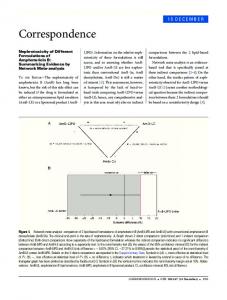
4 Results and discussion Fig. 1 (graph on the left) shows the centerline velocity in the startup flow problem, for different fluid parameters. Quite unlike newtonian fluids, which monotonically approach the assymptotic steady-state velocity distribution, the startup flow of viscoelastic fluids displays a variety of behaviours, including damped oscillations, overshoots and even localized backward motion. Some of these effects are displayed also in Fig. 1 (right), where the velocity profiles at different times for a fluid with E=3, β=0.01 are plotted. Similar general remarks hold relative to the pulsated flow problem, as shown in Fig. 2. We will examine in more detail different aspects of these results in the following subsections. '

&

& %

% !"#&%

$

$

,- ./0

+,-#.!&/

!"#

%$!"#$%!&$ !'#$%!&()$ !*#$%!&(&'$

#

!"#'%

#

!'"%

!

!

!"#(% !(#)%

"

"

!

!

!(#*%

!(#+%

"

#

% -

'

(

"

"'#

"'%

"'(

"')

!

/

Figure 1: Centerline velocity for the startup problem, for three different sets of parameters (left) and velocity profiles at different times for a fluid with E = 3, β = 0.01 (right). The lines plot the analytical solutions; the small circles show numerical results. Numerical results were obtained with the SPSS formalism, using a mesh with δy = 0.01, δt = 0.4δy (left) and δt = 0.2δy (right).

493

L. J. Amoreira and P. J. Oliveira / Adv. Appl. Math. Mech., 4 (2010), pp. 483-502 % $"#

() *+,

*+,#-!&.

#

!"

$ !"#

!"#$%!&$ !"#$%!&'&&" !(#$%!&'&)$

!"# !"$%&# !"$&# !"$'&#

! !"#

$

$!#

$!%

$!&

$!'

!

!"%

,

!"&

!"'

!"(

$

+

Figure 2: Centerline velocity in the pulsated flow problem, for three different parameter sets during one cycle of pulsation (left) and velocity profiles for E = 2, β = 0.001 at different instants (right). As in Fig. 1, lines represent analytical solutions, while the dots represent numerical results, obtained with δt = δy = 0.002 (left) and δt = δy = 0.001 (right).

4.1

Equivalence of formulations EVSS and EDIF

The different formulations are, of course, all analytically equivalent. Numerically, they differ in what is included in source terms. But formulations EVSS and EDIF have equal source terms for the Momentum Equation (1.22a). This can be seen either by noting that what is not a source term is the same in both algorithms or after expressing the equations in terms of a common stress tensor, like the original, physically measurable τ, for instance. The momentum equations in EDIF and EVSS are, therefore, fully equivalent, also in a numerical sense. Before we realized this, simulations of the same flow performed with the two formulations produced exactly the same results to all decimal digits, in exactly the same number of iterations. Retrospectively, this conclusion supports the justifications for the EDIF formulation presented in [8]. Being equivalent both analytically and numerically, there is really no point in testing separately the two formulations and, as such, we will give no further consideration to EDIF.

4.2

Convergence and stability

Generally, the methods tested are stable, in the sense that errors do not amplify in time. However, convergence of the iterative procedure in the ORIG formulation is difficult for β>0, especially in the initial stages of flow inception, unless a very small time integration step is used (typically, δt ∼0.01δy for β=0.1, both in the start-up and the pulsated flow problems). This difficulty demonstrates the need for stabilizing procedures such as those (generation of an explicit diffusive term) defined by the alternative formulations of the Oldroyd-B model generally adopted (e.g., EVSS) in numerical simulations that we consider in this work. But because of this convergence difficulty, the ORIG formulation is really only an option for UCM fluids, where convergence can be achieved with larger time steps.

494

L. J. Amoreira and P. J. Oliveira / Adv. Appl. Math. Mech., 4 (2010), pp. 483-502

Recall, however, that at β=0 formulations ORIG and SPSS are equivalent; even at that limit, then, there are no strong arguments to prefer the ORIG formulation over any other. For this reason, there is no point in further considering the ORIG method, and so in the remaining of this work only SPSS and EVSS are discussed. For all formulations (except ORIG) convergence is more difficult as β approaches zero. As was just mentioned, formulation SPSS approaches ORIG, as β→0, and because of this, for small enough β>0 some convergence difficulties also show up, forcing constraints on the time step. However, the situation is not as difficult as the one just described in the previous paragraph, and setting δt = 0.4δy, ensures convergence in most situations.

4.3 Accuracy As it is shown in Figs. 3 (for the start-up flow problem) and 4 (pulsated flow), the two formulations SPSS and EVSS produce essentially the same results. Differences in results obtained with different algorithms typically show up at the sixth or seventh significant digit. For a more quantitative assessment of numerical accuracy, we define the following measure of the error of a numerical solution at time t, based on the L2 norm of the difference relative to the analytical solution, h 1 ε(t) = Ny

Ny

∑

³ u j (t) − u

(a)

(t, y j )

´2 i 12

,

(4.1)

j =1

where Ny is the total number of control volumes (internal grid points). We can use a similar measure to estimate the discrepancy between numerical results obtained with

Figure 3: Analytical results (solid line) and computed with formulations SPSS (circles) and EVSS (crosses), for the start-up flow of a fluid with E = 1, β = 0 and for another with E = 5, β = 0.1. Velocity at the center of the channel (left) and shear stress at the margin (right) are plotted. The numerical results were computed with integration steps δy = 0.01, δt = 0.4δy.

L. J. Amoreira and P. J. Oliveira / Adv. Appl. Math. Mech., 4 (2010), pp. 483-502

495

Figure 4: Analytical results (solid line) and computed with formulations SPSS (circles) and EVSS (crosses), for the pulsated flow of a fluid with E = 1, β = 0 and for another with E = 5, β = 0.1. Velocity at the center of the channel (left) and shear stress at the margin (right) are plotted. Numerical results obtained with mesh parameters δy = 10−3 , δt = 0.5δy.

two different formulations. In Fig. 5, the discrepancy between results obtained for the start-up flow problem with formulations SPSS and EVSS is ploted together with the error e for SPSS, for an UCM fluid with E=1, using a mesh with 200 control volumes. This figure shows that the difference between numerical results from the two formulations is as much as four to five orders of magnitude lower then the error of either. Similar values are obtained considering different values of E and β, and also in the the pulsated flow problem. The different formulations are then indeed essentially indistinguishable regarding accuracy, in the sense that the discrepancy between them is always smaller than the discretization error. This conclusion was to be expected, since the main difference between formulations lies in different choices regarding which terms are treated as source terms and which are treated implicitly, that is, which terms enter the calculation with values computed in the previous iteration and which are computed afresh in each iteration. But the iterative process is such that, when converg-

!"#$%&'()(( ()(('*+((

,-.2

!"#

,-.1

,-.0

,-./

,-.,-

2

1

0

/

,-

"

Figure 5: Error of SPSS (relative to analytic results) and difference between SPSS and EVSS, both estimated as the L2 norm of the difference, in the start-up flow problem for an UCM fluid with E = 1, using a mesh with δy = 0.005, δt = 0.4δy.

496

L. J. Amoreira and P. J. Oliveira / Adv. Appl. Math. Mech., 4 (2010), pp. 483-502

ing, the differences between successive estimations of variable values become smaller and smaller. In the convergence limit, they vanish, and so do the differences between formulations. Different algorithms may follow different iterative paths to their predictions, but the predictions themselves, when they are reached, must be equal. Expectedly, the error gets lower as the integration steps δt and δy are reduced but, when keeping one of them constant and lowering the other, the first will eventually dominate and further reducing the value of the other integration step does not improve accuracy. For this reason, in studying the convergence rate of the algorithms, we always take the two integrations steps proportional to each other [5]. Figs. 6 and 7 display graphs of the error as a function of time, for several integration steps. !" !&!%'%($ !&!%'%"$ !&!%'%%)$ !&!%'%%()$ !&!%'%%"()$

!"#$ !%$

!"#$ !%&"

!"$

!'()

"*+,

!

"%

!"%

!"$

!"# !"# !"

!

%

#

&

+

'

!

!

!

&

%

$

#

!

(

Figure 6: Error as a function of time for different integration steps in the start-up flow problem for an UCM fluid with E = 1 (graph on the right, δt = 0.4δy was used) and for an Oldroyd-B fluid with E = 1, β = 0.1 (graph on the right, computed with δt = δy).

Since second-order approximations were used in the discretization of the governing equations, we expect the time average of the error (¯ε=∑ ε(tn )/Nt ) to be ideally given by ε¯ = c1 δy2 + c2 δt2 , for some real constants c1 and c2 . Taking δt proportional to δy, the average error should then be proportional to the second power of δy. However, this quadratic behavior is not always achieved. Instead, the error is in general a lower power r of δy, ε¯=c3 δyr . Fig. 8 displays plots of the average error for different fluids as a function of δy. Regarding the start-up flow problem (on the left), the convergence rates for UCM fluids are disappointingly around 1 (0.977 for E=1, similar results for other values of E with UCM fluid). However, for general Oldroyd-B fluids with β>0, the convergence rates rise up to around 2 (1.764, 1.981, 1.992 and 1.94 for β=0.001, 0.01, 0.1 and 0.9, respectively) and the error is indeed a quadratic function of the mesh parameter. The low convergence rates displayed by UCM fluids in the start-up flow problem are due to a discontinuity in the gradient of the shear stress that is generated at the margins of the channel at time t=0. At the margins, the no-slip condition sets d~v/dt=0. The momentum equation (1.1) then reduces to ~∂ · τ =~∂p. But the pumping ~∂p is suddenly

497

L. J. Amoreira and P. J. Oliveira / Adv. Appl. Math. Mech., 4 (2010), pp. 483-502 !"&

!!

!"#$ !%&%'

!" !"%

!"(

!()*

"*+,

!"' !"&

!"#"$ "#"% "#""& "#""$& "#""%$&

!"% !"$

!"$

!"# '!%()!!"

!"# !

!)(

!)&

!)$

!)*

!

!'&

+

!'$

!'(

!')

)

Figure 7: Like Fig. 6, but now for the pulsated flow problem. The graph on the left shows the error for an UCM fluid with E = 1, while the one on the right corresponds to an Oldroyd-B fluid with E = 1, β = 0.05. In all calculations a time step δt = δy was used.

!" !"'

!"%

'

&

!"& !"# !"$""%# !"$"%# !"$%# !"$&#

!"$

!"# !"$""%# !"$"%# !"$%# !%#

!"% !"$ !"#

!"# !"&

!"' ()

!"&

!"' '(

Figure 8: Average error ε¯ as a function of mesh parameter δy for E = 1. The lines plot best fits to a power function ε¯ = aδyr . Results for the start-up flow (left) were obtained with δt = 0.4δy; for the pulsated flow (right), δt = δy was used.

”turned on” at t=0, generating a discontinuity in the√stress gradient, which propagates back and forth across the channel with velocity E [5], without any dissipation mechanism for the case β=0. This generates a persistent discontinuity in the acceleration of the flow, visible in the graph of Fig. 1 (solid line, corresponding to β=0). Such temporal and spatial discontinuities are the cause for the much lower accuracy of calculations with β=0 displayed in Fig. 6 above and also for the lower convergence rates. In the pulsated flow problem, we extend the simulation for a long enough time period so that initial conditions (including the severe discontinuities just referred to) decay to negligible influence, as discussed in Section 3. For this reason, in pulsated flow simulations the accuracies of UCM fluid simulations are not much lower than those of general Oldroyd-B fluids and the convergence rates are in all cases, much closer to 2 (1.72 for β=0, 1.86, 1.97, 1.98 and 1.99 respectively for β=0.001, 0.01, 0.1 and 1), as can be seen in Fig. 8 (graph on the right).

498

L. J. Amoreira and P. J. Oliveira / Adv. Appl. Math. Mech., 4 (2010), pp. 483-502

4.4 Efficiency As shown in the previous section, the accuracy of all formulations is virtually the same. Regarding accuracy, then, all formulations are equivalent. However, different formulations converge to the results with widely varying numbers of iterations. We recall that, due to the decoupled nature of our algorithms, iterations are required inside each time step to deal with the inherent non-linearities and the inter-linkage between flow and constitutive equations. In practice, most algorithms in computational rheology, using either finite element or finite volume methods, are of decoupled nature and thus require iteration. For the present spatially one-dimensional problem, the algebraic equations [like Eq. (3.1)] are solved with the tridiagonal matrix algorithm TDMA, which is a direct solver. Therefore, the number of outer iterations within a time step are representative of the computational load along the simulation time and thus provide a transient measure of efficiency.

,-

!"#!$#%&'()&%!*+

!"#!$#%&'()&%!*+

,.--!" #"$""% #"$"% #"$% #"$&

,

,--

,-

, -

.

/

0

1

,-

-

/

0

1

2

,-

'

Figure 9: Number of iterations needed to achieve convergence as a function of time for the SPSS formulation (left) and for EVSS (right), for the start-up flow problem (E = 1). A mesh with δy = 0.01 and δt = 0.004 was used. Note the very different scales used in the two plots.

In Fig. 9, the numbers of iterations needed to achieve convergence in the start-up flow problem are displayed, for E=1 and different values of β, as functions of time. The graphs show clearly that, as discussed previously, convergence takes an increased numerical effort at the initial stages of flow inception and, in addition, as β→0. It is also clearly displayed in Fig. 9 that formulation SPSS is much more efficient than EVSS. The latter needs longer iterative cycles to converge in all situations. For small enough values of β, the number of iterations in EVSS may rise up to twenty times the SPSS value. The SPSS algorithm is also manifestly more efficient in the pulsated flow problem. As can be seen in Fig. 10, EVSS takes a number of iterations to converge up to two orders of magnitude larger then EVSS, especially so for small values of β. In addition, another negative aspect of EVSS relative to SPSS is that the number of iterations per time step shows a much larger sensitivity to the value of the retardation ratio β. SPSS

499

L. J. Amoreira and P. J. Oliveira / Adv. Appl. Math. Mech., 4 (2010), pp. 483-502 ,-0 !"# "$""%# "$"%# "$%# "$&#

,-/ !"#!$#%&'()&%!*+

!"#!$#%&'()&%!*+

,--

,-

,-.

,-, '((# )"# ,--

, -

-".

-"/

-"0

-"1

,

-

-".

-"0

-"1

-"2

,

*

Figure 10: Number of iterations needed to achieve convergence as a function of time in SPSS (left) and EVSS (right), for the pulsated flow problem (E = 1). All calculations done with δy = 0.001, δt = 0.5δy.

requires only about 3 iterations for all β6=0, while the iteration numbers for EVSS rise from ≈ 10 for β=0.5 to ≈ 60 at β=0.1, ≈ 200 at β=0.01, and even higher values as β→0. In Fig. 11, the total numbers of iterations needed to complete the simulations of the start-up flow up to non-dimensional time t=10 and of the pulsated flow during a complete period of the pressure gradient oscillation are plotted as functions of β, both for SPSS and EVSS. The ordinate in this graph is directly proportional to the overall computational work required to achieve a solution giving thus a direct measure of the relative efficiency of the two formulations. Again, we note that the iterative convergence is much more difficult for small β and that SPSS is in general more efficient then EVSS. But the most striking point in Fig. 11 is the fact that the efficiency of SPSS is essentially constant, independent of β, as already commented upon in the previous paragraph in relation to Fig. 10. By setting a variable (s= β) weight of the diffusive

/0!"+'1!-#"!102,

348 !"#!$%&' ( !"#!$%&')* (%+,"!-.' ( (%+,"!-.')*

347

346

345 4

49:

496

498

49;

3

Figure 11: Total numbers of iterations as a function of beta, for the start-up flow problem up to t = 10 (circles) and for the pulsated flow problem (triangles), for a complete period of the pressure oscillation. The meshes used here were the same as those for Figs. 9 (start-up flow) and 10 (pulsated flow).

500

L. J. Amoreira and P. J. Oliveira / Adv. Appl. Math. Mech., 4 (2010), pp. 483-502

term in the Momentum Equation [Eqs. (2.4a) and (2.13a)], the algorithm adjusts itself to the fluid under consideration, resulting in an efficient calculation even in the most difficult cases. 1-,--!"#$% !"#&% !"#'% !"#(%

0/,--!"#$%&"'(#"&!)*

0.,--0+,--01,--0-,--/,--.,--+,---

-21

-2+

-2.

-2/

0

)

Figure 12: Total number of iterations as a function of parameter s, for the start-up flow of four different Oldroyd-B fluids, with common E = 1 but varying β. The calculations were done using δy = 0.01, δt = 0.4δy.

This can be more clearly verified by measuring the workload (again, estimated by the total number of iterations) for different values of the weight of the added diffusive term (that is, the parameter s). We recall that in EVSS this parameter is unity, while for SPSS s= β. Fig. 12 displays plots of the total number of iterations in the startup flow problem (as in Fig. 11) as a function of s, for four different fluids. In all cases, there is a sharp reduction of the number of iterations needed to complete the calculation for s= β, that is, for the SPSS formulation.

5 Conclusions In this work different approaches to the numerical stabilization of the governing equations of the Oldroyd-B model were compared. The methods studied (Elastic-Viscous Stress Splitting, Solvent-Polymer Stress Splitting and Explicit Diffusion) are based on the inclusion of diffusive terms in the Momentum Equation, either redefining the stress tensor or compensating for the added terms in source terms, in such a way that the resulting governing equations are analytically (but not numerically) equivalent to the Oldroyd-B model. It was found that algorithms EDIF and EVSS are equivalent. It was also shown that, at least in the simple, one-dimensional problems considered, the approach based on solvent-polymer stress splitting is much more efficient then elastic-viscous stress splitting. Indeed, solvent-polymer stress splitting can be regarded as an adaptative EVSS, in the sense that the ”amount” of stress splitting is variable, depending on the

L. J. Amoreira and P. J. Oliveira / Adv. Appl. Math. Mech., 4 (2010), pp. 483-502

501

properties of the fluid being described (depends on β, specifically) in an optimal (regarding efficiency) way. Since many other more complicated models can be written under the same framework of the Oldroyd-B equations with the inclusion of additional ”source” terms, it is expected that the present findings may be extended to such models. In further investigations we will try to verify these findings in higher dimensional problems and to gain further insight on the conditions for optimal efficiency of this class of stabilization procedures.

References [1] M. G. P ERERA AND K. WALTERS, Long-range memory effects in flows involving abrupt changes in geometry, J. Non-Newton. Fluid., 2 (1977), pp. 49–81. [2] R AJAGOPALAN , R. A. B ROWN AND R. C. A RMSTRONG, Finite element methods for calculation of steady viscoelastic flow using constitutive equations with a Newtonian viscosity, J. Non-Newton. Fluid., 36 (1990), pp. 159–199. [3] J. S UN , N. P HAN -T HIEN AND R. I. TANNER, An adaptative viscoelastic stress splitting scheme and its applications: AVSS/SI and AVSS/SUPG, J. Non-Newton. Fluid., 65 (1996), pp. 76–91. [4] R. B. B IRD , R. C. A RMSTRONG AND O. H ASSAGER, Dynamics of Polymeric Liquids, Volume I, John Wiley & Sons, 1987. [5] A. R. S. D UARTE , A. I. P. M IRANDA AND P. J. O LIVEIRA, Numerical and analytical modeling of unsteady viscoelastic flows: the start-up and pulsating test case problems, J. Non-Newton. Fluid., 154 (2008), pp. 153–169. [6] R. G UNETTE AND M. F ORTIN, A new mixed finite element method for computing viscoelastic flows, J. Non-Newton. Fluid., 60 (1995), pp. 27–52. [7] P. J. O LIVEIRA , F. T. P INHO AND G. A. P INTO, Numerical simulation of non-linear elastic flows with a general collocated finite-volume method, J. Non-Newton. Fluid., 79 (1998), pp. 1–43. [8] M. A. A LVES , F. T. P INHO AND P. J. O LIVEIRA, Effect of a high-resolution differencing scheme on finite-volume predictions of viscoelastic flows, J. Non-Newton. Fluid., 93 (2000), pp. 278– 314. [9] J. G. O LDROYD, On the formulation of rheological equations of state, Proc. Roy. Soc. A., 200 (1950), pp. 523–541. [10] N. F ITIER AND M. O. D EVILLE, Time-dependent algorithms for the simulation of viscoelastic flows with spectral element methods: applications and stability, J. Comput. Phys., 186 (2002), pp. 93–121. [11] S.-C. X UE , R. I. TANNER AND N. P HAN -T HIEN, Numerical modelling of transient viscoelastic flows, J. Non-Newton. Fluid., 123 (2004), pp. 33–58. [12] M. A BOUBACAR , T. N. P HILLIPS , H. R. TAMADDON -J AHROMI , B. A. S NIGEREV AND M. F. W EBSTER, High-order finite volume methods for viscoelastic flow problems, J. Comput. Phys., 199 (2004), pp. 16–40. [13] R. G. M. VAN O S AND T. N. P HILLIPS, Spectral element methods for transient viscoelastic flow problems, J. Comput. Phys., 201 (2004), pp. 286–314. [14] N. D. WATERS AND M. J. K ING, Unsteady flow of an elastico-viscous liquid, Rheol. Acta., 9 (1970), pp. 345–355.

502

L. J. Amoreira and P. J. Oliveira / Adv. Appl. Math. Mech., 4 (2010), pp. 483-502

[15] T. H AYAT, A. M. S IDDIQUI AND S. A SGHAR, Some simple flows of an Oldroyd-B fluid, Int. J. Eng. Sci., 39 (2001), pp. 135–147. [16] J. M. K HODADADI , N. S. V LACHOS , D. L IEPSCH AND S. M ORAVEC, LDA measurements and numerical prediction of pulsatile laminar flow in a plane 90-degree bifurcation, J. Biomech. Eng., 110 (1988), pp. 129–136. [17] J. D. A NDERSON . J R ., Computational Fluid Dynamics, McGraw-Hill, 1995.