Comparison of iterative angular spectrum and optimal rotation angle methods in designing beam-fanners Seyyed H. Kazemi,1,2* Mir M. Mirsalehi,1 and Amir R. Attari1 2
1 Electrical Engineering Department, Ferdowsi University of Mashhad, Iran Communications and Computer Research Center, Ferdowsi University of Mashhad, Iran
[email protected]
Abstract: We compare the iterative angular spectrum (IAS) and the optimal rotation angle (ORA) methods in designing two-dimensional finite aperture diffractive optical elements (FADOEs) used as beamfanners. The transfer functions of both methods are compared analytically in the spatial frequency domain. We have designed several structures of 1-to-4 and 1-to-6 beamfanners to investigate the differences in the performance of the beamfanners designed by ORA method for near field operation. Using the three-dimensional finite difference time-domain (3-D FDTD) method with perfect matched layer (PML) absorbing boundary condition (ABC), the diffraction efficiency is calculated for each designed FADOE and the corresponding values are compared. © 2009 Optical Society of America OCIS codes: (050.1970) Diffractive optics; (050.1220) Aperture; (000.4430) Numerical approximation and analysis
References and links 1. 2. 3. 4. 5. 6. 7. 8. 9.
10. 11. 12. 13.
J. Jiang, and G. P. Nordin, “A rigorous unidirectional method for designing finite aperture diffractive optical elements,” Opt. Express 7(6), 237–242 (2000). D. W. Prather, M. S. Mirotznik, and J. N. Mait, “Boundary integral methods applied to the analysis of diffractive optical elements,” J. Opt. Soc. Am. A 14(1), 34–43 (1997). D. W. Prather, J. N. Mait, M. S. Mirotznik, and J. P. Collins, “Vector-based synthesis of finite aperiodic subwavelength diffractive optical elements,” J. Opt. Soc. Am. A 15(6), 1599–1607 (1998). J. W. Goodman, Introduction to Fourier Optics (Roberts & Company, Englewood, 2005). J. Bengtsson, “Design of fan-out kinoforms in the entire scalar diffraction regime with an optimal-rotationangle method,” Appl. Opt. 36(32), 8435–8444 (1997). J. Stigwall, and J. Bengtsson, “Design of array of diffractive optical elements with inter-element coherent fan-outs,” Opt. Express 12(23), 5675–5683 (2004). R. W. Gerchberg, and W. O. Saxton, “Practical algorithm for the determination of phase from image and diffraction plane pictures,” Optik (Stuttg.) 35, 237–250 (1972). F. Wyrowski, and O. Bryngdahl, “Iterative Fourier-transform algorithm applied to computer holography,” J. Opt. Soc. Am. A 5(7), 1058–1065 (1988). F. Di, Y. Yingbai, J. Guofan, T. Qiaofeng, and H. Liu, “Rigorous electromagnetic design of finite-aperture diffractive optical elements by use of an iterative optimization algorithm,” J. Opt. Soc. Am. A 20(9), 1739– 1746 (2003). T. G. Jabbour, and S. M. Kuebler, “Vectorial beam shaping,” Opt. Express 16(10), 7203–7213 (2008). S. D. Mellin, and G. P. Nordin, “Limits of scalar diffraction theory and an iterative angular spectrum algorithm for finite aperture diffractive optical element design,” Opt. Express 8, 706–722 (2001). D. M. Sullivan, “An unsplit step 3-D PML for use with the FDTD method,” IEEE Microwave and Guided Wave Letters 7(7), 184–186 (1997). D. M. Sullivan, Electromagnetic Simulation Using the FDTD Method, IEEE Press series on RF and microwave technology, 2000.
1. Introduction Several methods have been used to design diffractive optical elements (DOEs). These methods can be generally divided to unidirectional and bidirectional methods. The unidirectional methods combine the analysis of DOE with optimization techniques. Examples of analysis methods are scalar phase only approximation and rigorous electromagnetic methods such as finite difference time domain (FDTD) [1] and boundary element method [2, 3]. The analysis methods often use additional methods to model the #110959 - $15.00 USD Received 4 May 2009; revised 1 Jul 2009; accepted 24 Jul 2009; published 6 Aug 2009
(C) 2009 OSA
17 August 2009 / Vol. 17, No. 17 / OPTICS EXPRESS 14825
wave propagation from the output plane (the plane just behind the DOE) to the observation plane, e.g. Fresnel and Fraunhofer propagation approach or angular spectrum (AS) approach [4]. The optimization methods, such as micro-genetic [1] or simulated annealing [3], search the space of unknown DOE parameters using fitness function. Another unidirectional method is the optimal rotation angle (ORA) [5, 6]. In this method, the phase of each cell in the DOE is changed to maximize the intensities at a limited number of spots. In bidirectional methods, analysis and inverse-analysis are used iteratively to improve the DOE structure. Gerchberg–Saxton method [7], iterative Fourier transform algorithm (IFTA) [8], the method proposed by Di [9], vectorial beam shaping by Jabbour [10] and iterative angular spectrum algorithm (IASA) [11] are various kinds of bidirectional methods. The Gerchberg–Saxton method and the IFTA method are used for far and near field cases. The method proposed by Di uses FDTD and thin element approximation (phase only approximation) as analysis and inverse-analysis methods, respectively and AS approach for wave propagation simulation. In the IASA, the optical field in the output plane is calculated using phase only approximation. This field is then propagated to the observation plane by AS approach. In this paper, we compare the IAS and ORA methods in designing FADOEs as 2-D beamfanners. Since the original IAS method was presented for 1-D case, we have extended it for the 2-D case. The extended iterative angular spectrum (IAS) method is described in section 2 that is followed by a description of the ORA method. The transfer functions of these methods are compared in section 4. Both methods, as well as the FDTD method, are used to design and analyze 1-to-4 and 1-to-6 beamfanners in section 5 which is followed by conclusions. 2. Iterative angular spectrum method The geometry of a 2-D finite aperture DOE is shown in Fig. 1. The input plane that includes the aperture is located in front of the DOE and the observation plane is located at z=zobs. It is assumed that a plane wave propagating along the z-axis interacts with the DOE at the input plane and it is expected to produce the desired pattern at the observation plane. The space between the input and the observation plane is divided to two regions: DOE region and AS region. The DOE region extends from the input plane to the output plane (P0) and includes DOE, while the AS region extends from the output plane located at z=0 to the observation plane (P1). The thickness of DOE region is equal to the maximum etch depth (dmax). The refraction index of the dielectric material used is n2, while the surrounding medium is assumed to be air (n1=1). The transmission function of the DOE is
t(x,y) = τ exp[jφ ( x, y )]Π ( x / L x , y / L y ),
(1)
where τ=2n1/(n1+n2) is Fresnel transmission coefficient, Π(x/Lx, y/Ly) is equal to 1 for any point inside a rectangular aperture of Lx×Ly, and equal to zero for other points. The phase function according to phase only approximation is φ(x,y)=k0∆nd(x,y), where ∆n is the difference between the two refractive indices, k0=2π/λ, λ is the wavelength in free space and d(x,y) is the etch depth. We assume an incident plane wave, uinc, that is propagating normal to the aperture. The wave at the output plane of the first region is u0=t(x,y)uinc. The angular spectrum of u0, i.e., U0, is defined as [4]
#110959 - $15.00 USD Received 4 May 2009; revised 1 Jul 2009; accepted 24 Jul 2009; published 6 Aug 2009
(C) 2009 OSA
17 August 2009 / Vol. 17, No. 17 / OPTICS EXPRESS 14826
Fig. 1. Geometry of 2D finite aperture DOE and the two regions used in the IAS method.
U 0 ( f x , f y ) = ∫∫ u 0 ( x, y ) exp[− j 2π ( f x x + f y y )]dxdy.
(2)
P0
Using the fast Fourier transform (FFT) technique, U0 can be computed. Assuming a square aperture, Lx=Ly=L, the distance between two adjacent points in spatial frequency domain is δf=δfx=δfy=1/L. To improve the resolution in the frequency domain, we can compute the FFT on an area larger than the DOE area. This is particularly useful if the desired intensity profile in the observation plane extends beyond the DOE area. The field distribution in the observation plane, u1, can be obtained by u1 ( x, y ) = ∫
∞
∫U
0
exp[ jk2 z obs 1 − (λ2 f x ) 2 − (λ2 f y )2 ]exp[ j 2π ( f x x + f y y )]df x df y , (3)
−∞
where k2=n2k0 and λ2=λ/n2 are the wave-number and wavelength in the AS region, respectively [4]. Using the inverse fast Fourier transform (IFFT), u1 can be calculated as u1=IFFT(HU0), where H(f x , f y ) = exp[ jk2 z obs 1 − (λ2 f x )2 − (λ2 f y ) 2 ]
(4)
is the angular spectrum transfer function. The maximum spatial frequency is fmax=1/(2δ), where δ is the minimum feature size of the DOE. To consider all propagating waves, the condition fmax>1/λ2, which is equivalent to δ