comparison of linear and nonlinear statistics methods applied in ...

Serbian Journal of Management 5 (2) (2010) 189 - 198

Serbian Journal of Management

www.sjm06.com

COMPARISON OF LINEAR AND NONLINEAR STATISTICS METHODS APPLIED IN INDUSTRIAL PROCESS MODELING PROCEDURE Predrag Đorđević, Ivan Mihajlović* and Živan Živković University of Belgrade, Technical faculty in Bor Vojske Jugoslavije 12, 19210 Bor, Serbia (Received 10 May 2010; accepted 10 June 2010) Abstract This paper presents the comparison of Multiple Linear Regression Analysis (MLRA) and Artificial Neural Networks (ANN) as the statistical analysis tools. Most influential statistical parameters for choosing right modeling tool are evaluated in this investigation. Investigation was performed on real statistical data set obtained after measurements of the process parameters underindustrial conditions. Keywords:MLRA, ANN, statistical modeling

1. INTRODUCTION The main objective of this study was to investigate applicability and constrains of the linear (MLRA) and nonlinear (ANN) methods of statistical analysis. Both approaches were used for modeling the same data set obtained during experiment facilitated under the industrial conditions. The technological process that was the target of this investigation was aluminate solution decomposition, as the part of the Bayer alumina production process. However, technological process in question is not that * Corresponding author: [email protected]

much of interest in this paper. This paper is focused on the methodological process of modelling. Same methodological approach could be used for many other industrial processes. In the process which was modeled in these investigations, following input variables were considered: concentration of the Na2O (caustic); caustic ratio and crystallization ratio; starting temperature; final temperature; average diameter of crystallization seed and duration of decomposition process. Only one output variable was correlated above defined inputs

P.\or|evi} / SJM 5 (2) (2010) 189 - 198

190

of the process. Output variable considered was the degree of the aluminate solution decomposition.

2. MODELING PROCEDURE In the contemporary systems theory literature, two main modeling approaches could be distinguished: M1 – modeling procedure based on the system of differential equations resulting from cognizance of the systems structure and interdependence among the elements of the system (Weir, 1991; Brown, 2007; Dragićević and Bojić, 2009). M2 – modeling procedure based on experimentally obtained data on the output of the system, resulting after introduction limited set of selected input parameters of the process (Taylor et al., 2003; Giraldo – Zuniga et al., 2006). In this paper modeling approach M2 was selected. M2 approach could further be divided on analytical and statistical methods. For modeling described in this paper we used statistical methods, both linear (MLRA) and nonlinear (ANNs).

3. STARTING DATA SET For modelling the process of aluminate solutions decomposition the data from thefactory Birač, Zvornik (Bosnia and Hercegovina), were used. The data was collected during the years 2008 - 2009, by measuring input and output process parameters, under stable operation mode of the production line. Total number of 500 data sets was collected this way, comprising: a) Input parameters of the process: Na2O (caustic) content in the solution (g/dm3) – X1; caustic ratio (αk) of the solution – X2; crystallization ratio – X3; starting temperature of the solution (oC) – X4; final temperature of the solution (oC) – X5; average diameter of the crystallization seed (μm) – X6; and the duration of the crystallization process (h) – X7. b) Output parameter of the process: degree of decomposition of the solution (%) – Y.

Table 1. Values of the input (Xi) and the output (Y) variables of the process of industrial sodium aluminate solution decomposition – descriptive p p statistics of 500 data sets Mean Range X1 X2 X3 X4 X5 X6 X7 Y

12.3 0.2 3.4 11.0 22.2 37.7 76.0 24.3

Minimum 144.0 1.5 1.3 58.0 36.3 87.2 49.0 32.3

Maximum 156.3 1.7 4.7 69.0 58.5 124.9 125.0 56.6

Statistic 150.944 1.530 2.285 64.656 50.582 106.473 77.080 46.658

Std. Error 0.0762 0.0015 0.0296 0.0536 0.1839 0.3806 0.6236 0.1241

Std. Deviation 1.7030 0.0329 0.6617 1.1988 4.1121 8.5098 13.9437 2.7747

Variance 2.900 0.001 0.438 1.437 16.909 72.416 194.426 7.699

P.\or|evi} / SJM 5 (2) (2010) 189 - 198

191

considerable increase of rate and the degree of decomposition of the solution. For example, if X2 is changed from 1.7 to 1.5,

4. RESULTS AND DISSCUSION

Values of the measured input parameters the degree of decomposition (Y) will of the technological process (X1 – X7) and increase from 51% to 55%, with all other the process quality indicator – output of the input parameters kept constant. For definition of the correlation process (Y) in the form of descriptive statistics results, are presented in table 1. dependence in the form: output of the It can be noticed that variable X2 has process (Y) = f input of the process (X1 – quite small variance (see Table 1). Nevertheless, this variable presents the caustic ratio of the solution and it is one of the most important parameters of the Bayer process. This way it shouldn’t be omitted from subsequent analyse. Even small decrease of this variable leads to

X7), bivariate correlation analysis was performed. As the result of this analysis Pearson Correlation (PC) coefficients with responding statistical significance were calculated, Table 2. To finally define the dependence of the output parameter as the function of the input

Table 2. Correlation matrix for the input (X1 – X7) and the output (Y) variables of the industrial sodium aluminate solution dissociation process (number of data points for each variable is equal toq500) ) X1

X2

X3

X4

X5

X6

X7

Y

X1

Pearson Correlation Sig. (2-tailed)

1

X2

Pearson Correlation Sig. (2-tailed)

-.319** .000

1

X3

Pearson Correlation Sig. (2-tailed)

-.149** .001

.361** .000

1

X4

Pearson Correlation Sig. (2-tailed)

-.150** .001

.209** .000

-.030 .500

1

X5

Pearson Correlation Sig. (2-tailed)

.090* .045

-.252** .000

-.489** .000

.214** .000

1

X6

Pearson Correlation Sig. (2-tailed)

.115** .010

-.084 .061

.458** .000

-.040 .372

.066 .139

1

X7

Pearson Correlation Sig. (2-tailed)

-.125** .005

.159** .000

.421** .000

-.156** .000

-.716** .000

-.147** .001

1

Y

Pearson Correlation Sig. (2-tailed)

-.143** .001

.073 .101

.447** .000

-.108* .016

-.720** .000

-.227** .000

.661** 1 .000

**. Correlation is significant at the 0.01 level (2-tailed). *. Correlation is significant at the 0.05 level (2-tailed).

P.\or|evi} / SJM 5 (2) (2010) 189 - 198

192

parameters, using the multiple linear regression analysis (MLRA) with acceptable level of fitting (strong correlation), it is necessary that the value of PC is near 0.5 with statistical significance (p ≤ 0.05) (Moroney, 1998; Živković et al., 2009a; Živković et al., 2009b). Analysis of the data presented in the Table 2 reveals that this constraint is attained in following cases: Y – X3 : PC = 0.447 (p = 0.000); Y – X5 : PC =

data base and it was used for testing of the model. Linear dependence of degree of analysed solution decomposition (Y) on influencing parameters of the technological process (X1X7) was obtained using SPSS software application Version 17.0 (SPSS Inc, 2010). The complete linear model, developed during training of the model, is as follows:

- 0.720 (p = 0.000); Y – X7 : PC = 0.661 (p Y = 102.864 – 0.044.X1 – 23.108.X2 + = 0.000). This was also the case for the . . . . following interdependence between the 1.817 X3 + 0.140 X4 – 0.297 X5 – 0.136 X6 predictors of the process: X3 – X5 : PC = - + 0.027.X (R2 = 0.670) (1) 7 0.489 i p = 0.000; X7 - X5: PC = -0.716 i p = 0.000; X6 – X3 : PC = 0.458 i p = 0.000; The results of the ANOVA tests of developed model are presented in Table 3. X7 – X3 : PC = 0.421 i p = 0.000. Significant F statistics (see Table 3) is Considering that there is a considerable indicating that using the model is better then number of variables with acceptable level of guessing the mean. Also, the significance correlation and statistical significance (p ≤ value of the F statistic is less than 0.05 which 0.05), it was concluded that the MLRA means that the variations explained by the approach should be considered as the model are not due the chance. Regression adequate tool for modelling of investigated displays information about the variation process. For the purpose of MLRA analysis, accounted for by the model, residual displays the assembly of 500 input and output data information about the variation that is not sets was divided into two groups. First group accounted for by the model. The ratio of consisted 350 (70%) of randomly selected regression to residual is 67%: 33%, data lines, and it was used for training of the advocating that 67% of the dependent model, while the second group consisted 150 variable (Y) values are explained by the (30%) remaining data lines from the starting model. Table 3. Results of ANOVAa,b test performed during training of the model Model Regression

Sum of Squares 1772.337

df 7

Mean Square 253.191

874.209

342

2.549

2646.546

349

Residual Total

a. Predictors: (Constant), X7, X4, X6, X2, X1, X5, X3 b. Dependent Variable: Y

F 99.341

Sig. 0.000a

P.\or|evi} / SJM 5 (2) (2010) 189 - 198

Results describing MLRA model summary, for the training phase, are presented in the table 4. The multiple correlation coefficient (R) is presenting the linear correlation between the observed and model-predicted values of the dependent variable. Its large value (0.818) indicates a strong relationship. R square, the coefficient of determination, is the squared value of the multiple correlation coefficient. It shows that about 67% of variation in Y is explained by the model, as already indicated by the regression to residual ratio. As the future measure of the strength of the model fit, we compared the standard error of the estimate in the model summary table (Table 4) to the standard deviation of Y reported in the descriptive statistics table (Table 1). Without prior knowledge of the X1– X7 values, our best guess for the Y would be about 46.65% with standard deviation of 2.77. With the MLRA model the error of our estimate is considerably lower, about 1.59%. Considering above model parameters, the model developed according to MLRA seemed highly acceptable for prediction of the gibbsite crystallisation under the industrial conditions. On the other hand, after running the collinearity analysis of the models coefficients, the results obtained showed that Table 4. MLRA summarya,b of the model developed during the training phase

Model 1

R 0.818a

R Square 0.670

Adjusted R Square 0.663

Std. Error of the Estimate 1.5965

a. Predictors: (Constant), X7, X4, X6, X2, X1, X5, X3 b. Dependent Variable: Y

193

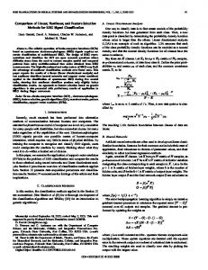
there might be a problem with multicollinearity of the model. For most predictors, the values of the partial and part correlations drop sharply from the zero-order correlation (see Table 5). This means, for example, that much of the variance in Y that is explained by X2 is also explained by other variables. The tolerance is the percentage of the variance in a given predictor that cannot be explained by the other predictors. Thus, relatively small tolerances in case of predictors X3, X5 and X7 show that more than half of the variance in a given predictors can be explained by the other predictors. A variance inflation factor (VIF) greater than 2 is usually considered problematic and in the example modelled in this paper; this is the case for predictors X3, X5 and X7. Also, important factor of the collinearity analysis is condition index. Values of condition index greater then 15 indicate a possible problem, with collinearity greater than 30 a serious problem. Five of these indices were larger then 30, in case of this example, suggesting a very serious problem with collinearity. We tried to fix this collinearity problem by running the regression using stepwise method of model selection, hoping that most of the predictors will remain in the final model. Unfortunately, this did not improve the collinearity situation. However, after developing the model in the training stage, validation of the model was performed in the testing stage using the second part of the data base (total 150 vectors). During the testing phase of the MLRA model, calculated coefficient of determination (R2) was slightly increased in comparison to the testing phase and now it equals: 0.731. Figure 1 illustrates comparative presentation of the measured and the values calculated using the MLRA

P.\or|evi} / SJM 5 (2) (2010) 189 - 198

194

Fig. 1. Dependence between calculated and measured values of the caustic sodium aluminate solutions degree of decomposition ( - ideal position; --- regression lines; o valuescalculated using MLRA model in the testing stage) approach for the investigated process. As presented in previous text, better fit was obtained on the test set than on the training set. This suggests that most of the extreme points that are more difficult to model are in the training set. The selection of the variables

for the training and the testing stage was performed using random number generator and it was not subjectively influenced. Also, all the data lines were examined for potential outliers before the MLRA. Strong extreme behaviour of the variables was not detected.

Table 5. Results of collinearity analysis of the MLRA model Correlations Model 1

Collinearity Statistics

Zero-order

Partial

Part

Tolerance

VIF

X1

-0.158

-0.043

-0.025

0.834

1.200

X2

0.072

-0.375

-0.233

0.702

1.425

X3

0.416

0.433

0.276

0.415

2.407

X4

-0.078

0.098

0.057

0.894

1.119

X5

-0.699

-0.452

-0.292

0.434

2.303

X6

-0.266

-0.484

-0.317

0.579

1.726

X7

0.649

0.161

0.094

0.443

2.256

P.\or|evi} / SJM 5 (2) (2010) 189 - 198

195

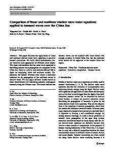
This way, obtained results are the true parameters of the connections is achieved represent of the investigated process. through necessary number of iterations, until the mean squared error between the 4.1. Artificial neural networks calculated and measured outputs of the network is minimal. During the second The ANN used in the model development phase, the remaining 20 – 30% of the data is is depicted in Fig.2. As shown, this network used for testing of the ’’trained’’ network. In consists of three layers of nodes. The layers this phase, the network is using the weighted described as input, hidden and output layers, parameters determined during the first phase. can generally comprise (i), (j) and (k) This 20 – 30% of the data, excluded during number of processing nodes, respectively. the learning of the network, is now Each node in the input (hidden) layer is incorporated in it as a new input values Xi linked to all the nodes in the hidden (output) which is then transformed to the new outputs layer using weighted connections. In Y . The third phase is the validation of the i addition to the (i) and (j) number of input and network on completely new data set. This hidden nodes, the ANN architecture also data set is usually consisting of the data from houses a bias node (with fixed output + 1) in new experimental measurements of the same its input and hidden layers and they provide process. The validation phase is presenting additional adjustable parameters (weights) the final level of successful or unsuccessful for the model fitting. The number of the predicting using the network developed in nodes (i) in the ANN network input layer is the previous two stages, on future database equal to the number of inputs in the (Živković et al., 2009; Liu et al., 2009). processwhereas the number of output nodes Same as in the MLRA procedure, the (k) equals the number of the process outputs. assembly of 500 input and output data sets However, the number of hidden nodes (j) is was divided into two groups. First group an adjustable parameter magnitude of which consisted 350 (70%) of randomly selected is determined by issues, such as the desired data lines, and it was used for training of the approximation and generalization network, while the second group consisted capabilities of the network model (Zeng, et 150 (30%) remaining data lines from the al., 1997). starting data base and it was used for testing The back propagation algorithm modifies of the network. network weights to minimize the mean For development of relational ANN squared error between the desired and the configuration we used previously defined actual outputs of the network. Back input parameters X1 – X7 and output propagation uses supervised learning in which the input, as well as desired outputs parameter Y (degree of decomposition of are controlled and selected (Eberhart and sodium aluminate solution), as the elements of the network architecture, Figure 2. Dobbins, 2002). The appropriate number of neurons in the The use of ANN usually comprises hidden layer was determined by training threephase. First is the training phase which is facilitated on 70 to 80% randomly selected several networks. This is necessary because data from the starting data set. During this of the fact that too low number of neurons in phase the correction of the weighted the hidden layer produces high training and

196

P.\or|evi} / SJM 5 (2) (2010) 189 - 198

Fig. 2. The ANN architecture for determination of the degree of decomposition of the sodium aluminate solution as the function of input process parameters testing errors due to under-fitting and statistical bias. On the contrary, too many hidden layer neurons lead to low training error, but high testing error, due to overfitting and high variance. Because of this, in this study, we used the iterative approach to determine the optimal number of hidden layer neurons, yielding minimum model prediction error on the “test data set”. This way, we have tested 13 networks, ranging from 2 to 14 neurons in the hidden layer. The best results were obtained with the network architecture presented in Fig.2. In the phase of training of the network, for each of the network architectures, necessary

number of iteration was performed, until the error between the measured output of the decomposition process of industrial sodium aluminate solution Y- and calculated values was minimized and remained constant. After developing of this kind of ’’trained’’ network, testing stage was performed using the second part the data base (total 150 vectors). In this phase also, all 13 hidden layer structures were involved, until obtaining minimum model prediction error. The ANN structure presented in Fig. 2, with seven neurons in the hidden layer, resulted with minimum model prediction error. For such network, obtained coefficient of

P.\or|evi} / SJM 5 (2) (2010) 189 - 198

197

Fig. 3. Comparison of the measured and the values calculated using ANN for prediction of the degree of industrial sodium aluminate solution dissociation -Y determination is R2 = 0.762 for the training industrial data collected in this study can be phase. During the ANN testing phase, used for the purpose of predicting gibbsite crystallization. However, the model calculated coefficient of determination (R2) developed cannot be used for optimization of was slightly increased in comparison of the the process, since optimization requires testing phase and now it equals: 0. 895. cause and effect relationships of the data Figure 3 illustrates comparative presentation which can only be obtained through of the measured and the values calculated orthogonal design of experiments (DOE) and using the ANN approach for investigated not from normal production data, because of process. The same situation happened as in the collinearity of the variables (see Table 2 the MLRA approach, meaning that better fit and Table 5). was obtained on the test set than on the training set. The explanation for this is the same as in the case of MLRA modelling, References suggesting that most of the extreme points that are more difficult to model are in the Dragićević, S, Bojić, M., (2009) training set. Application of linear programming in energy management, Serbian Journal of Management 4 (2): 227 - 238. 5. CONCLUSIONS Eberhart, R.C., Dobbins, R.W. (2002) Neural Network PC Tools: A Practical Results obtained indicate that the

P.\or|evi} / SJM 5 (2) (2010) 189 - 198

198

Guide, Academic, New York. Giraldo-Zuniga, A.D., Arevalo-Pinedo, A., Rodrigues, R.M., Lima, C.S., Feitosa, A.C. (2006) Kinetic drying experimental data and mathematical model for jackfruit slices, Cienc. Technol. Aliment., 5(2): 89-92. Liu, D., Yuan, Z., Liao, S. (2009) Artificial neural network vs. nonlinear regression for gold content estimation in pyrometallurgy, Expert Systems with Applications, 36: 10397 – 10400. Moroney, R.N. (1998) Spurious of virtual correlation errors commonly encountered in reduction of scientific data, Journal of Wind Engineering and Industrial Aerodynamics, 77&78: 543-553. SPSS inc. PASW Statistics 18, Predictive Analysis Software Portfolio, www.spss.com Taylor, C.F., Paton,N.W., Garwood, K.L. (2003) A systematic approach to modeling, capturing, and disseminating proteomics experimental data, Nature Biotechnology 21 : 247 - 254.

Weir G. (1991) Differential Equations - A Modeling Approach, Addison-Wesley, Hardcover. Brown, C. (2007) Differential Equations A Modeling Approach, Sage Publications. Zeng, J., Yin, Z., Chen, Q. (1997) Intensification of precipitation of gibbsite from seeded caustic sodium aluminate liquor by seed activation and addition of crown ether, Hydrometallurgy, 89:107 – 116. Živković, Ž., Mihajlović, I., Nikolić, Dj. (2009) Artificial neural network method applied of the nonlinear multivariante problems, Serbian Journal of Management, 4(2): 137 – 149. Živković, Ž., Mitevska, N., Mihajlović, I., Nikolic, Đ. (2009) The influence of the silicate slag composition on copper loses during smelting of the sulfide concentrates, Journal of Mining and Metallurgy 45 B: 2335.

ПОРЕЂЕЊЕ МЕТОДА ЛИНЕАРНЕ И НЕЛИНЕАРНЕ СТАТИСТИКЕ ЗА МОДЕЛОВАЊЕ ИНДУСТРИЈСКИХ ПРОЦЕСА Предраг Ђорђевић, Иван Михајловић, Живан Живковић Универзитет у Београду, Технички факултет у Бору, Одсек за менаџмент

Извод У овом раду је приказан однос вишеструке линеарне регресије (МЛРА) и вештачких неуронских мрежа (АНН) у статистичкој анализи. Наиме, показани су најутицајнији параметри на основу којих се може донети одлука да ли експерименталне податкке треба моделовати употребом линеарне статистичке анализе МЛРА или нелинеарне статистичке процедуре АННс. Испитивање је урађено на реалном статистичком скупу добијеном мерењем процесних параметара у индустријским условима. Кључне речи: МЛРА, АНН, моделовање