Quantitative evaluation of linear and nonlinear methods characterizing
Recommend Documents
visualize a sequence of numbers being written on a blackboard, and rotate a 3-dimensional ..... http://theoval.sys.uea.ac.uk/Ëgcc/svm/toolbox. University of East ...
in contexts that differ from their textbooks. This paper gives a short introduction to the general linear model (GLM), in which it is showed that ANOVA (one-way, ...
Deon Garrett, David A. Peterson, Charles W. Anderson, and. Michael H. Thaut ... gram, Colorado State University, Fort Collins, CO 80523 USA (e-mail:.
Abstract. This paper presents the comparison of Multiple Linear Regression Analysis (MLRA) and ... Serbian Journal of Management 5 (2) (2010) 189 - 198.
Abstract. This paper presents the comparison of Multiple Linear Regression Analysis (MLRA) and ... performed on real statistical data set obtained after measurements of the process parameters .... X7) was obtained using SPSS software.
frequently used to determine the best-fitting isotherm) and nonlinear (which ... isotherm selection, a comparison of linear and nonlinear regression methods was.
http://www.statistik.tuwien.ac.at. Linear and nonlinear methods for regression and
classification and applications in R. P. Filzmoser. Forschungsbericht CS-2008- ...
I. INTRODUCTION. UMERICAL shell structures analysis became popular ... International Science Index, Civil and Environmental Engineering Vol:7, No:2, 2013 ...
Blecker & Friedrich/ MASS CUSTOMIZATION: Challenges and Solutions. Appa,
Pitsoulis & Williams/ ... Printed on acid-free paper. 987654321 springer.com ...
separate parts. Part I is a self-contained introduction to linear programming, a key
.
Whilst others had shown that a wave can be represented as ... independent spatial variables x â Rn, where n is generally equal to 1, 2 ... an oscillation that travels through a medium by transferring energy from one particle or point to ... Rossby
tive function is separable with respect to the two groups of variables. The augmented ..... approximation. Skill in modeling, to capture the essential elements of a problem, ... of constraints and objectives that arise in practice are indisputably li
The last two parts together comprise the subject of nonlinear programming. ...
have elegant and potent theories and for which effective algorithms are avail-
able.
I would like to thank my advisor, Professor David R. Williams for his guidance and help as ... Force Office of Scientific Research Grant FA9550-12-1-0075. iii ... 3.2 Peak value of â CL dependence on single-pulse pulse width, α = 20o, ..... The ex
1.4 Matrix splittings and classical stationary iterative methods . . 7. 1.5 Exercises
on ... 3.8 Examples for CGNR, Bi-CGSTAB, and TFQMR iteration . . . 55.
Nov 29, 2006 - Barry D. Cookson,1 D. Ashley Robinson,2 Alastair B. Monk,3 Stephen Murchan,4 Ariane Deplano,5. Rafaël de Ryck,5 Marc J. Struelens,5 ...
CV] 5 Feb 2016 ... results are discussed in Section 5. Finally the main findings and future directions ... ered by 5 different methods (i.e., 32Ã5Ã2 = 320 minutes).
Feb 21, 2017 - context of DTI, the results might generalize to fMRI studies that ... complete analysis pipeline, exploiting the idea that in the ideal acquisition ...
ABSTRACT: Previously, we developed an integrated software package called ... as a spatial technique for characterizing remote ...... cal assistance. dimensions.
models. These models were also utilized to select the most efficient subsets of descriptors in a cross-validation procedure for non-linear log (1/EC50) prediction.
This thesis develops two Bayesian learning methods relying on Gaussian .....
error loss for regression problems and 0/1-loss for classification; others will be ...
Nov 11, 2002 - 2437. PAPER. Linear and Nonlinear Lagrange Relaxation Algorithms for ... On one hand, a path selection algorithm for the QoS routing must be ...... munications Letters and the IEEE Network, a technical editor of the IEEE ...
Vanderbei/ LINEAR PROGRAMMING: Foundations & Extensions, 3rd Edition.
Chhajed ... Part I is a self-contained introduction to linear programming, a key.
May 19, 2015 - Y. Jiang, Dr. D. Gindre, M. Allain, Dr. C. Cabanetos,. Prof. J. Roncali ... emission of light or exciton diffusion are for a large part controlled by intermo- ..... [31] F. Würthner , T. E. Kaiser , C. R. Saha-Möller , Angew. Chem. I
Thanks also to all staff members of the Department of Applied Physics and. Centre for Research and ..... greatly differ from that of conventional materials (Indolia and Gaur 2013) . The ..... different techniques by (Gupta et al. 2006).Moreover,the .
Quantitative evaluation of linear and nonlinear methods characterizing
Quantitative evaluation of linear and nonlinear methods characterizing interdependencies between brain signals Karim Ansari-Asl, Lotfi Senhadji,* Jean-Jacques Bellanger, and Fabrice Wendling INSERM U 642, Laboratoire Traitement du Signal et de L’Image, Université de Rennes 1, Campus de Beaulieu, 35042 Rennes Cedex, France 共Received 28 September 2005; revised manuscript received 6 June 2006; published 26 September 2006兲 Brain functional connectivity can be characterized by the temporal evolution of correlation between signals recorded from spatially-distributed regions. It is aimed at explaining how different brain areas interact within networks involved during normal 共as in cognitive tasks兲 or pathological 共as in epilepsy兲 situations. Numerous techniques were introduced for assessing this connectivity. Recently, some efforts were made to compare methods performances but mainly qualitatively and for a special application. In this paper, we go further and propose a comprehensive comparison of different classes of methods 共linear and nonlinear regressions, phase synchronization, and generalized synchronization兲 based on various simulation models. For this purpose, quantitative criteria are used: in addition to mean square error under null hypothesis 共independence between two signals兲 and mean variance computed over all values of coupling degree in each model, we provide a criterion for comparing performances. Results show that the performances of the compared methods are highly dependavxx on the hypothesis regarding the underlying model for the generation of the signals. Moreover, none of them outperforms the others in all cases and the performance hierarchy is model dependent. DOI: 10.1103/PhysRevE.74.031916
Brain functional connectivity is defined as the way different brain areas interact within networks involved during normal 共as in cognitive tasks兲 or pathological 共as in epilepsy兲 activity. It can be characterized by the temporal evolution of the cross correlation 共in a wide sense兲 between signals recorded from spatially distributed regions. During the past decades, numerous techniques have been introduced for measuring this correlation. In the early fifties, the first developed methods 关1兴 were based on the cross-correlation function and its counterpart in the frequency domain, i.e., the coherence function 关2,3兴 just after fast Fourier transform 共FFT兲 algorithms were introduced 关4兴. Some other methods based on a similar concept but using time-varying linear models to estimate the cross correlation were introduced later and were used to characterize the relationship between brain oscillations in the time and/or frequency domain 关5,6兴. As the aforementioned methods are mostly linear, recently a considerable number of studies have been dedicated to the development of nonlinear methods 关7兴, mostly because of the nonlinear nature of mechanisms at the origin of electroencephalographic 共EEG兲 signals. A family of methods based on mutual information 关8兴 or on nonlinear regression 关9,10兴 was first introduced in the EEG field. Another family is currently developing, based on works related to the study of nonlinear dynamical systems and chaos 关11,12兴. The latter family can be divided into two groups: 共i兲 phase synchronization 共PS兲 methods 关13,14兴 which first estimate the instantaneous phase of each signal and then compute a quantity based on
covariation of extracted phases to determine the degree of the relationship; 共ii兲 generalized synchronization 共GS兲 methods 关15,16兴 which also consist of two steps, in the first one, state space trajectories are reconstructed from scalar time series signals and in the second one, an index of similarity is computed to quantify the similarity between these trajectories. Given the number and the variety of methods introduced for characterizing brain signal interactions and considering the diversity of situations in which these methods are applied, there is a need for identifying objectively, among available methods, those which offer the best performances. Recently, some efforts have been made for comparing methods but mainly qualitatively 关17,18兴 and for particular applications 关19,20兴. In this paper, we go further and propose a comprehensive comparison of the aforementioned classes of methods 共linear and nonlinear regression, phase synchronization, and generalized synchronization兲 based on various simulation models 共linearly correlated noises, nonlinear coupled oscillators, and coupled neuronal population models兲 in which a coupling parameter can be tuned. Methods are compared according to quantitative criteria: 共i兲 the mean square error 共MSE兲 under null hypothesis 共independence between the two analyzed signals兲; 共ii兲 the mean variance 共MV兲 computed over all values of the coupling parameter in each model; 共iii兲 in addition to two preceding criteria, we proposed a criterion related to the method sensitivity. The paper is organized as follows: Sec. II introduces simulation models and briefly reviews some of the methods widely used in the field of EEG to estimate the degree of relationship between two signals. The results are presented in Sec. III and discussed in Sec. IV.
FIG. 1. General finite dimensional state-space model 共composed of two coupled subsystems S1 and S2兲 with three inputs N1, N2, N3 and two outputs x, y. Models considered in this study correspond to simplified versions of this model. See text for details. II. METHODS A. Models
In this section general features of models considered in this study are introduced. Each of them is a more or less simplified version of a general finite dimensional state-space model with three inputs and two outputs. This general model denoted by M CX,Y is decomposed in two subsystems S1 and S2 as illustrated in Fig. 1. To describe state evolution 共on discrete time or on continuous time兲 of the global system two finite dimensional marginal state vectors, respectively, denoted X and Y, must be introduced. In an EEG measurement perspective, X and Y macroscopically represent dynamical states of two functionally interdependent neuronal subpopulations, respectively. Each subsystem is specified by a state evolution equation: X共t + 兲 = FC„X共t兲; v共兲,t 艋 艋 t + …,X共t兲 苸 Rm , Y共t + 兲 = GC„Y共t兲;w共兲,t 艋 艋 t + …,Y共t兲 苸 Rn , where matrix C = 共Ci,j兲 is a matrix of positive numbers interpreted in the sequel as a coupling parameter which weights the effect of “nonautonomous” terms v and w, respectively, on states X and Y 共Fig. 1兲. The inputs N1, N2, and N3 are mutually independent, zeromemory, zero-mean, and unit-variance stochastic processes 共white noises兲 which can be interpreted, in a physiological perspective, as influences from distant neural populations. Input N3 corresponds to a possible shared afference. The scalar outputs x and y, in the same perspective, correspond to two EEG channels. If it exists, the dynamical “coupling” between states X and Y is represented through a functional dependence of v on Y and on the shared input N3 and through the dependence of w on X and N3: v共t兲 = g1„C1,1,N1共t兲,N3共t兲,Y共t兲…,
w共t兲 = g2„C2,1,N2共t兲,N3共t兲,X共t兲….
g1, g2, h1, and h2 are deterministic functions. The measurement noises, if present, are modeled by two independent random processes m1共t兲 and m2共t兲. If v does not depend on Y共·兲 and w does not depend on X共·兲 and if furthermore N3 = 0, then the two subsystems S1 and S2 are disconnected. In this case and when inputs N1 and N2 are present, outputs x and y are statically independent if h1 共respectively, h2兲 is not a function of Y 共respectively, X兲. Then equations become x共t兲 = h1(X共t兲) and y共t兲 = h2(Y共t兲), in the absence of measurement noise. The dashed lines in Fig. 1 correspond to the influences of S2 on the signal x. These influences are not considered in the present study 共neither a feedback influence of X on Y nor a forward influence of Y on x兲 except for one model 共the model denoted by M 1 hereafter兲. This consideration corresponds to a causal influence directed from S1 to S2 and clearly does not address the most general bidirectional situation which is beyond the scope of this paper. Consequently, matrix C is the parameter which tunes the dependence of y on X. When C is null no dependence exists. Dependence between the two systems is expected to increase with C coefficients. Depending on the model type, for large values of these coefficients and when N2 = 0 and m2 = 0, output y becomes a deterministic function of state X and of N3. In order to comprehensively simulate a wide range of coupled temporal dynamics we used various mathematical models as well as a physiologically relevant computational model of EEG simulation from coupled neuronal populations. Motivations for the choice of these kinds of relationship models in the context of brain activity are discussed in a previous work 关21兴. Degenerated model M 1 is derived by setting C1,1 = C2,1 = c and by letting the other matrix coefficient equal to zero with x = X = v and y = Y = w. This model generates two broadband signals 共x , y兲 from the mixing of the two independent white noises 共N1 , N2兲 with the common noise 共N3兲: x = 共1 − c兲N1 + cN3 , y = 共1 − c兲N2 + cN3 , where 0 艋 c 艋 1 is the coupling degree; for c = 0 the signals are independent and for c = 1 they are identical. In model M 2, the general description above reduces to: v = N1, w = N2, x = h1共X兲, C2,3 = c, and y = h2共X , Y , c兲. The other coefficients of the matrix C are all equal to zero. In practice, four low-pass filtered white noises 共F1, F2, F3, and F4兲 are combined in two ways to generate two narrowband signals around a frequency f 0. Generated signals share either a phase relationship 共PR兲 or an amplitude relationship 共AR兲, only:
The models for the two output scalar signals are: PR:
x共t兲 = h1„X共t兲,Y共t兲,m1共t兲…, 031916-2
再
x = A1 cos共2 f 0t + 1兲, y = A2 cos共2 f 0t + c1 + 共1 − c兲2兲,
冎
PHYSICAL REVIEW E 74, 031916 共2006兲
QUANTITATIVE EVALUATION OF LINEAR AND…
AR:
再
x = A1 cos共2 f 0t + 1兲, y = 共cA1 + 共1 − c兲A2兲cos共2 f 0t + 2兲,
冎
where A1 = 冑F21 + F22, A2 = 冑F23 + F24, 1 = arctan共 F21 兲, 2 F = arctan共 F43 兲, and 0 艋 c 艋 1. For c = 0, the two generated signals have independent phase and amplitude and for c = 1, they have identical phase or amplitude. We also evaluated interdependence measures on coupled temporal dynamics obtained from two models of coupled nonlinear oscillators, namely the Rössler 关22兴 and Hénon 关23兴 deterministic systems. In model M 3, where two Rössler systems 关24兴 are coupled, the driver system is F
dx1 = − xx 2 − x 3 , dt dx2 = xx1 + 0.15x2 , dt dx3 = 0.2 + x3共x1 − 10兲, dt and the response system is dy 1 = − y y 2 − y 3 + c共x1 − y 1兲, dt dy 2 = y y 1 + 0.15y 2 , dt dy 3 = 0.2 + y 3共y 1 − 10兲, dt here x = 0.95, y = 1.05, and c is the coupling degree. For this model, C2,1 = c 共other Ci,j are equal to zero兲, v = N1 = N2 = N3 = 0, w = g2共X , c兲 and the outputs are linear forms of the state vectors: x = h1共X兲 = HX and y = h2共Y兲 = HY. In model M 4, we used two Hénon maps to simulate a unidirectional coupled system. The Hénon map 关25兴 is a nonlinear deterministic system which is discrete by construction. Here, the driver system is x关n + 1兴 = 1.4 − x2关n兴 + bxx关n − 1兴, and the response system is y关n + 1兴 = 1.4 − „cx关n兴y关n兴 + 共1 − c兲y 2关n兴… + by y关n − 1兴, where c is a coupling degree and bx = 0.3; to create different situations, once by is set to 0.3 to have two identical systems 共M 4a兲 and once by is set to 0.1 to have two nonidentical systems 共M 4b兲. For each of these two cases 共identical or different systems兲, we added some measurement noise to verify the robustness of estimators against changes in signal-to-noise ratio 共S/N兲, here we evaluated the noise-free case 共S / N = inf.兲 and S / N = 2. S/N was computed as the ratio of standard deviation 共Std兲 of the signal over the Std of the noise. In this
case, this model matches the general description figure with C2,1 = c, v = N1 = N2 = N3 = 0, w = g2共X , c兲, x = h1共X兲 = HX + m1, and y = h2共Y兲 = HY + m2. Finally, to further match dynamics encountered in real EEG signals, especially in epilepsy, we considered a physiologically relevant computational model of EEG generation from a pair of coupled populations of neurons 关26兴. Each population contains two subpopulations of neurons that mutually interact via excitatory or inhibitory feedback: main pyramidal cells and local interneurons. The influence from neighboring is modeled by an excitatory input p共t兲 共i.e., here N1 or N2兲 that globally represents the average density of afferent action potentials 共Gaussian noise兲. Since pyramidal cells are excitatory neurons that project their axons to other areas of the brain, the model accounts for this organization by using the average pulse density of action potentials from the main cells of a first population as an excitatory input to a second population of neurons. A connection from a given population i to a population j is characterized by parameter Kij which represents the degree of coupling associated with this connection. Other parameters include excitatory and inhibitory gains in feedback loops as well as an average number of synaptic contacts between subpopulations. Appropriate setting of parameters Kij allows for building systems where neuronal populations can be unidirectionally and/or bidirectionally coupled. In model M5, we considered the case of two populations of neurons unidirectionally coupled 共K12 = c is varied and K21 stays equal to 0兲. This model was used to generate two kinds of signal: background 关M 5共BKG兲兴 and spiking 关M 5共SPK兲兴 EEG activity. For both cases, the normalized coupling parameter was varied from 0 共independent situation兲 to 1 value under which temporal dynamics of signals stay unchanged. Following the general description of the simulation model we have, C2,1 = c, v = N1, w = g2共X , c , N2兲 = N2 + cHX, N3 = 0, x = h1共X兲 = HX, and y = h2共Y兲 = HY. Here, HX and HY are linear forms of the state vectors. B. Interdependence measures and coupled systems
In an experimental context, the classical approach to evaluate a functional coupling between two systems S1 and S2 is a two step procedure. The first step consists of building an indicator of relationship between state vectors X and Y. The second step focuses on the estimation of the indicator as a function of the two outputs x and y observed over a sliding window of fixed length. The window length is set so that the observed signals are locally stationary. A naïve approach is to reduce this functional coupling to the value of parameter C in a given model M CX,Y , and hence to restrict the characterization to an estimation of this parameter. Indeed a value of C is not a definitive answer to the problem. The link, in a given model, between this value and the joint dynamical activity of coupled systems is generally not simple to establish theoretically. However, in some particular cases it can be derived analytically 共see Appendix A兲. Even in the case where we have an exact mathematical model M CX,Y allowing to accurately simulate the joint evolution of state vectors X and Y, it can be hard to closely analyze the functional rela-
031916-3
PHYSICAL REVIEW E 74, 031916 共2006兲
ANSARI-ASL et al.
tionship between them. The difficulty is that a general definition of a functional relationship index r共M CX,Y 兲 from X to Y, which should be taken as an “absolute reference,” does not exist 共a particular definition will generally capture only some cross-dynamical features兲. Furthermore a theoretical definition is not sufficient. It is also necessary to make a measurement from output signals x and y, i.e., to build an estimator rˆ共x , y兲 of r共M CX,Y 兲. In a model identification approach a natuˆ ˆ 共x , y兲 is an ral estimator should be rˆ共x , y兲 = r共M C共x,y兲兲 where C X,Y
estimation of C in model M CX,Y . This model based approach is beyond the scope of this paper. Our concern here is essentially to compare various coupling functionals R共x , y兲 defined directly on a pair of scalar observation signals without explicit reference to an underlying model. In this study, compared functionals and corresponding estimators Rˆ共x , y兲 are those widely used in the literature 共see Sec. II C兲. These measures can be considered as descriptive methods. C. Evaluated interdependence measures
We investigated the most widely used methods for characterizing stationary interactions between systems. These may be divided into three categories: 共i兲 linear and nonlinear regression: Pearson correlation coefficient 共R2兲, coherence function 共CF兲, and nonlinear regression 共h2兲; 共ii兲 phase synchronization: Hilbert phase entropy 共HE兲, Hilbert mean phase coherence 共HR兲, wavelet phase entropy 共WE兲, and wavelet mean phase coherence 共WR兲; 共iii兲 generalized synchronization: three similarity indexes 共S , H , N兲 and synchronization likelihood 共SL兲. Here we review succinctly their definitions. 共i兲 For two time series x共t兲 and y共t兲, Pearson correlation coefficient is defined in the time domain as follows 关27兴: R2 = max
兩xy共f兲兩2 =
where g共·兲 is a function which approximates the statistical relationship from x共t兲 to y共t兲. 共ii兲 Phase synchronization estimation consists of two steps 关13兴. The first step is the instantaneous phase extraction of each signal and the second step is the quantification of the degree of synchronization via an appropriate index. Phase extraction can be done by different techniques. Two of them are used in this work: the Hilbert transform and the wavelet transform. Using the Hilbert transform, analytical signal associated to a real time series x共t兲 is derived: H
ix 共t兲 , Zx共t兲 = x共t兲 + iH关x共t兲兴 = AH x 共t兲e H where H, H x , and Ax 共t兲 are, respectively, the Hilbert transform, the phase, and the amplitude of x共t兲. Complex continuous wavelet transform can also be used to estimate the phase of signal 关32兴:
Wx共t兲 = 共 * x兲共t兲 =
兩Sxy共f兲兩2 , Sxx共f兲 · Syy共f兲
冉
h2xy = max 1 −
冊
var„y共t + 兲/x共t兲… , var„y共t + 兲…
冕
W
ix 共t兲 共t⬘兲x共t − t⬘兲dt⬘ = AW , x 共t兲e
W where , W x , and Ax 共t兲 are, respectively, a wavelet function 共e.g., Morlet used here兲, the phase, and the amplitude of x共t兲. Once phase extraction is performed on the two signals under analysis, several synchronization indexes can be used to quantify the phase relationship. In this study, we explored two of them both based on the shape of the probability density function 共pdf兲 of the modulo 2 phase difference 关 = 共x − y兲mod2兴. The first index is stemmed from Shannon entropy and defined as follows 关33兴:
=
where Sxx共f兲 and Syy共f兲 are, respectively, the power spectral densities of x共t兲 and y共t兲, and Sxy共f兲 is their cross-spectral density. It is the counterpart of R2 in the frequency domain and can be interpreted as the squared modulus of a frequency-dependent complex correlation coefficient. Among nonlinear regression analysis methods, we chose a method introduced in the field of EEG analysis by Lopes da Silva and colleagues 关29兴 and more recently evaluated in a model of coupled neuronal populations 关30兴. Based on the fitting of a nonlinear curve by piecewise linear approximation 关31兴, this method provides a nonlinear correlation coefficient referred to as h2:
where
g
cov2„x共t兲,y共t + 兲… , var„x共t兲…var„y共t + 兲…
where var, cov, and denote, respectively, variance, covariance, and time shift between the two time series. The magnitude-squared CF can be formulated as 关28兴:
where M is the number of bins used to obtain the pdf, pi is the probability of finding the phase difference within the ith bin, and Hmax is given by ln M. The second index which is named mean phase coherence corresponds to 兩E关ei兴兩 and is estimated in 关34兴 by:
冏
N−1
冏
1 R= 兺 ei共t兲 , N t=0 where N is the length of time series. Combining two ways of phase extraction and two indices for quantification of phase relationship, we obtain four different measures of interdependencies: HE, HR, WE, and WR. 共iii兲 Generalized synchronization is also a two step procedure. First, a state space trajectory is reconstructed from each scalar time series using a time delay embedding method 关35兴. This technique makes it possible to investigate the interaction between two nonlinear dynamical systems without any knowledge about governing equations. First, for each discrete time n a delay vector corresponding to a point in the state space reconstructed from x is defined:
031916-4
PHYSICAL REVIEW E 74, 031916 共2006兲
QUANTITATIVE EVALUATION OF LINEAR AND…
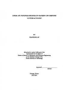
FIG. 2. Results obtained in model M 1 共stochastic broadband signals兲, using Monte Carlo simulation for Pearson correlation coefficient 共R2兲 CF兲, nonlinear regression 共h2兲, HE, Hilbert mean phase coherence 共HR兲, wavelet phase entropy 共WE兲, and wavelet mean phase coherence 共WR兲, three similarity indexes 共S , H , N兲 and 共SL兲. 共a兲 Simulated signals generated by model M 1, 共b兲 estimated relationships and 共c兲 variances of estimation.
Xn = 共xn,xn+, . . . ,xn+共m−1兲兲,n = 1, . . . ,N,
k
where m is the embedding dimension and denotes time lag. The state space of y is reconstructed in the same way. Second, synchronization is determined via a suitable measure. Four measures, all based on conditional neighborhood, are presented in this study. The principle is to quantify the proximity, in the second state space, of the points whose temporal indices are corresponding to a neighboring points in the first state space. Three of these measures S, H, and N 关15兴, which are also sensitive to the direction of interaction, originate from this principle and use an Euclidean distance:
R共k兲 n 共X兩Y兲 =
1 兺 兩Xn − Xsn,j兩2 , k j=1
where 兩·兩 is the Euclidean distance; rn,j , j = 1 , . . . , k and sn,j , j = 1 , . . . , k, respectively, stand for the time indices of the k nearest neighbors of Xn and Y n. The fourth measure, referred to as the SL 关16兴, is a measure of multivariate synchronization. Here we only focus on the bivariate case. The estimated probability that embedded vectors Xn are closer to each other than a distance is,
N
R共k兲 1 n 共X兲 , S 共X兩Y兲 = 兺 共k兲 N n=1 Rn 共X兩Y兲
Px,n
共k兲
1 = 2共w2 − w1兲
N
兺
共 − 兩Xn − X j兩兲
j=1
w1⬍兩n−j兩⬍w2 N
H共k兲共X兩Y兲 =
1 兺 log N n=1
R共N−1兲 共X兲 n , R共k兲 共X兩Y兲 n
N
R共N−1兲 共X兲 − R共k兲 1 n 共X兩Y兲 n N 共X兩Y兲 = 兺 , 共N−1兲 N n=1 Rn 共X兲 共k兲
where R共k兲 n 共X兲 is computed
where stands for Heaviside step function, w1 is the Theiler correction, and w2 determines the length of the sliding win = Py,n = Pref be a small arbitrary probability, dow. Letting Px,n the above equation for Xn and its analogous for Y n, gives the critical distances x,n and y,n from which we can determine if simultaneously Xn is close to X j and Y n is close to Y j, i.e., Hn,j = 2 in the equation below Hn,j = 共x,n − 兩Xn − X j兩兲 + 共y,n − 兩Y n − Y j兩兲.
k
R共k兲 n 共X兲 and R共k兲 n 共X 兩 Y兲 is
1 = 兺 兩Xn − Xrn,j兩2 , k j=1
Synchronization likelihood at time n can be obtained by averaging over all values of j, 031916-5
PHYSICAL REVIEW E 74, 031916 共2006兲
ANSARI-ASL et al. N
1 Sn = 2Pref 共w2 − w1兲
兺
共Hn,j − 1兲.
j=1
w1⬍兩n−j兩⬍w2
All aforementioned measures but H, are normalized between 0 and 1; the value of 0 means that the two signals are completely independent. On the opposite, the value of 1 means that the two signals are completely synchronized. D. Comparison criteria
For all models and all values of the degree of coupling parameter, long time series were generated in order to address some statistical properties of the computed quantities: 共i兲 the MSE under null hypothesis 共i.e., independence between two signals兲, which could be interpreted as a quadratic bias, defined by E兵共ˆ 0 − 0兲2其 where E is the mathematical expectation, 0 = 0 and ˆ 0 is the estimation of 0; 共ii兲 the MV computed over all values ci, i = 1 , 2 , . . . , I of the degree of I E兵共ˆ i − E共ˆ i兲兲2其 where I is numcoupling and defined as 1I 兺i=1 ber of coupling degree points and ˆ i is the estimated relationship for the coupling degree ci; 共iii兲 in addition to two above criteria, we introduced the median of local relative sensitivity 共MLRS兲 as a comparison criterion, it given by: MLRS = Median共Si/¯i兲,
Si =
ˆ i+1 − ˆ i , ci+1 − ci
¯i =
冑
2 ˆ 2i + ˆ i+1 , 2
where Si is the increase rate of the estimated relationship and ¯i is the square root of the average of estimated variances associated to two adjacent values of the coupling degree. This quantity is a reflection of the sensitivity of a method with respect to the change in the coupling degree. We have also retained the median of the distribution of local relative sensitivity instead of its mean because the fluctuation in its estimation may make this distribution very skewed. Contrary to MSE and MV, higher MLRS values indicate better performances. For all models and all values of the degree of coupling, Monte Carlo simulations were conducted to compare interdependence measures provided by methods described in Sec. II C. For the parameter used in the GS methods, first the mutual information as a function of positive time lag is plotted and then as described in 关36兴 the time lag was chosen as the abscissa value corresponding to the first minimum this curve. The embedded dimension m, in these kinds of methods, was determined from the Cao method 关37兴. Appendix B provides details about the implementation of the methods
III. RESULTS
Mean value and variance for each coupling degree are shown in Figs. 2–7 for all methods except H that does not provide normalized quantity. For model M 1 共Fig. 2兲, all quantities but N reach the value of 1 for c = 1. R2 and h2 methods behave very similarly because the relationship in M 1 is completely linear.
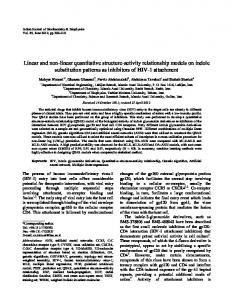
Regarding phase synchronization measures, we observed a similar method behavior as curves were found to be very close to one another. For signals generated with model M 1, SL was also found to have the maximum variance among all measures particularly for the high values of the coupling parameter, as depicted in Fig. 2共c兲. This result was not expected because the variance generally falls for the high relationship degree. Finally, we also observed in M 1 that S and CF have nonnegligible MSE under null hypothesis compared to other measures. The results obtained in model M 2 are shown in Fig. 3. For PR only 关Figs. 3共a兲–3共c兲兴, we observed that PS methods exhibit higher performances than other methods as expected. Similarly, R2 and h2 methods gave rather good results. On the opposite, GS methods and coherence had lower performances. In the case of AR only 关Figs. 3共d兲–3共f兲兴, PS methods did not present any sensitivity to changes in the degree of relationship as expected from their definitions. GS, R2, and h2 methods provided quantities which slightly increase with an increasing degree of coupling. Finally, despite what is commonly thought, CF showed only slight sensitivity to amplitude covariation. In this study, nonlinear deterministic systems 共models M 3 and M 4兲 were used only for comparing the performances of relationship estimators. Their properties were not investigated in detail here as they have already been analyzed in many previous studies 关38兴. For the two coupled Rössler systems 共Fig. 4兲, we found that the SL method had both the least MSE under the null hypothesis and the best sensitivity with respect to change in the coupling degree. However, its variance stayed high compared to other methods. Qualitatively, PS methods performed better in this case. A striking result was also obtained in this case: several methods 共R2, h2, and WE兲 provided quantities which first increased and then decreased for increasing low values of the coupling parameter 共0 ⬍ c ⬍ 0.14兲. For coupled identical Hénon systems 共M 4a兲, N performed better than other methods 共Fig. 5兲. For nonidentical Hénon systems 共M 4b兲, GS methods still exhibited the best performances 共Fig. 6兲. Although MSE and MV were found to be reduced with the addition of measurement noise for all methods, it is worth mentioning that regression methods are generally more robust against noise than other approaches, especially for nonidentical coupled systems. For the neuronal population model 共model M 5兲, signals were generated to reproduce normal background EEG activity 关M 5共BKG兲兴 or spiking activity 关M 5共SPK兲兴 as observed during epileptic seizures. Properties of these signals are very close to those reported in a previous attempt for comparing relationship estimators 关17兴. In our study, the relationship between the two modeled populations of neurons was unidirectional. As shown in 关18兴 in the case of background activity using surrogate data techniques, the relationship between signals in this model are mainly linear. Thus we expected all methods to exhibit similar behavior in this case. Results showed that increasing the degree of coupling between neuronal populations did not lead to a significant increase of computed quantities, as shown in Figs. 7共a兲–7共c兲. In this situation CF and all the PS methods but HR do not detect any relationship; other methods detect a weak relationship. For
031916-6
PHYSICAL REVIEW E 74, 031916 共2006兲
QUANTITATIVE EVALUATION OF LINEAR AND…
FIG. 3. Results obtained in model M 2 共stochastic narrowband signals兲. 共a兲 Simulated signals generated by model M 2共PR兲, 共b兲 estimated relationships, and 共c兲 variances of estimation, for the PR case. 共d兲–共f兲 Results for the AR case.
spiking activity, results for all methods are reported in Figs. 7共d兲–7共f兲. As an interesting result, we observed that WE and CF were almost blind to the established relation. Similarly, HE and WR only displayed a small increase with an increasing of degree of coupling but their variance was low. R2, h2, S, methods exhibited good sensitivity. However, MSE under null hypothesis was found to be high for HR. Results presented in Figs. 1–6 are summarized in Tables I–III which, respectively, give the MSE under null hypothesis, the MV and the MRLS for all methods and simulation
models 共see Appendix C for the confidence intervals兲. For each studied situation, the best method is indicated with bold face characters. Methods that were found to be insensitive with respect to changes in the coupling degree are denoted by the symbol “*.” From these tables, we deduced that for model M 1, R2 is the most appropriate estimator based on defined criteria. For model M 2, in the case of phase relationship, PS methods 共especially WE兲 perform better than other methods. In the case of amplitude relationship, there is no consensus for the choice of a best method as all methods are
031916-7
PHYSICAL REVIEW E 74, 031916 共2006兲
ANSARI-ASL et al.
FIG. 4. Results obtained by model M 3 共Rössler coupled systems兲. 共a兲 Simulated signals, 共b兲 estimated relationship and 共c兲 variances of estimation.
more sensitive to the phase of signals than to their envelope. For the coupled Rössler systems 共M 3兲, PS methods are more suitable. For Hénon coupled systems, S and N methods had higher performances, on average but R2 was found to be more robust in the presence of added noise. For the neuronal population model, in the background activity situation, R2 and h2 methods detected the presence of a relationship and performed better than other methods; this tendency was also confirmed in the spiking activity situation. However, it was difficult to determine the overall best method in this second case since criteria did not lead to consensual results. In order to globally compare the three groups of methods, we averaged results obtained in each simulation model for each criterion. Results are synthesized in Fig. 8. For model M 1, regression methods perform better than others as the MV is the lowest while the MRLS is the highest. For model M 2 共in the case of PR兲, it is evident that PS methods are the most appropriate. For model M 2 共in the case of AR兲, there is no consensus for the best method. For model M 3, PS methods outperform others although they are characterized by higher MSE values. For model M 4 共considering the four situations兲, GS methods have the lowest MSE and PS methods have the lowest MV. As far as the MRLS is concerned, these two groups of methods perform equally. Finally, for the neuronal population model M 5, regression methods outperform others in the case of normal background EEG activity. For spiking epilepticlike activity, these methods, in addition to PS methods have also higher performances than GS methods. IV. DISCUSSION AND CONCLUSIONS
Numerous methods have been introduced to tackle the difficult problem of characterizing the statistical relationship
between EEG signals without any a priori knowledge about the nature of this relationship. This question is of great interest for understanding brain functioning in normal or abnormal conditions. Therefore, these methods play a key role as they are supposed to give important information regarding brain connectivity from electrophysiological recordings. In this work, we compared the performances of various estimators for quantifying statistical coupling between signals and characterizing interactions between brain structures. We analyzed, quantitatively and as comprehensively as possible, various kinds of estimators using different models of relationship for representing the wide range of signal dynamics encountered in brain recordings. In this regard, our study differs from that of Schiff et al. 关39兴 who evaluated one method to characterize dynamical interdependence 共based on mutual nonlinear prediction兲 on both simulated 共coupled identical and nonidentical chaotic systems as those used here兲 and real 共activity of motoneurons within a spinal cord motoneuron pool兲 data. It also differs from other evaluation studies which mainly focused on qualitative comparisons 关17,18兴 and for particular applications 关19,20兴. In the particular field of EEG analysis, the model of coupled neuronal populations is of particular relevance since it generates realistic EEG dynamics. In this model, for background activity 共that can be considered as a broadband random signal兲, we found that coherence and phase synchrony methods 共except HR兲 were not sensitive to the increase of the coupling parameter whereas regression methods 共linear and nonlinear兲 exhibited better sensitivity. This result may be explained by the fact that the interdependence between simulated signals is not entirely determined by a phase relationship. This point is crucial since it illustrates the fact that the
031916-8
PHYSICAL REVIEW E 74, 031916 共2006兲
QUANTITATIVE EVALUATION OF LINEAR AND…
FIG. 5. Results obtained for model M 4a 共identical Hénon coupled systems兲. 共a兲 Simulated signals generated by model M 4a共S / N = inf, the noise-free case兲, 共b兲 estimated relationship, and 共c兲 variances of estimation, for the noise-free case. 共d兲–共f兲 Results for the S / N共signal-to noise ratio兲 = 2 case.
choice of the method used to characterize the relationship between signals is critical and may lead to possible misleading interpretation of EEG data. In addition, as background activity can be recorded in epileptic patients during interictal periods, our results also relate to those recently published by Morman et al. 关19兴 in the context of seizure prediction. For thirty different measures obtained from univariate and bivariate approaches, au-
thors evaluated their ability to distinguish between the interictal period and the preseizure period 共sensitivity and specificity of all measures were compared using receiveroperating characteristics兲. In both types of approach 共and consequently for bivariate methods similar to those implemented in the present study兲 they also found that linear methods performed equally good or even better than nonlinear methods.
031916-9
PHYSICAL REVIEW E 74, 031916 共2006兲
ANSARI-ASL et al.
FIG. 6. Results obtained for model M 4b 共nonidentical Hénon coupled systems兲. 共a兲 Simulated signals generated by model M 4b共S / N = inf, the noise-free case兲, 共b兲 estimated relationship, and 共c兲 variances of estimation, for the noise-free case. 共d兲–共f兲 Results for the S / N共signal-to-noise ratio兲 = 2 case.
Moreover, we did not report results about the capacity of some measures to characterize the direction of coupling in some models 共in particular in asymmetrically coupled oscillators or neuronal populations兲. This issue which is beyond the scope of the present study has already been addressed in other reports. For instance, Quian Quiroga et al. 关40兴 quantitatively tested two interdependence measures on coupled
nonlinear models 共similar to those used here兲 for their ability to determine if one of the systems drives the other. To sum up, the main findings of this study are the following: 共i兲 some of the compared methods are insensitive to particular signal coupling; 共ii兲 results are very dependent on signal properties 共broad band versus narrow band兲; 共iii兲 generally speaking, there is no universal method to deal with
031916-10
PHYSICAL REVIEW E 74, 031916 共2006兲
QUANTITATIVE EVALUATION OF LINEAR AND…
FIG. 7. Results obtained for model M 5 共neuronal population model兲. 共a兲 Simulated signals by model M 5共BKG兲, 共b兲 estimated relationship, and 共c兲 variances of estimation, for the background activity. 共d兲–共f兲 Results for the spiking activity case.
signal coupling, i.e., none of the studied methods performed better than the other ones in all studied situations; 共iv兲 as R2 and h2 methods showed to be sensitive to all relationship models with average or good performances in all situations. This latter point led us to conclude that it is reasonable to apply R2 and h2 methods as a first attempt to characterize the functional coupling in studied systems in absence of a priori information about its nature. In addition, in the case where
such information is available, this study can help to choose the appropriate method among those studied here. ACKNOWLEDGMENTS
One of the authors 共K.A.兲 gratefully acknowledges the scholarship from the Iranian ministry of science, research, and technology and supports from the LTSI, the University
031916-11
PHYSICAL REVIEW E 74, 031916 共2006兲
ANSARI-ASL et al.
TABLE I. MSE values and standard deviations 共see Appendix C for computation兲 for studied methods and models. “*” denotes methods that are nearly insensitive to changes in the coupling degree and for which this criterion is not applicable.
of Rennes I and the INSERM, received during his Ph.D. thesis research.
In the ideal case, analytical expression of R共x , y兲 as a function of coupling parameter values is required to compute MSE. Generally, this analytical expression cannot be obtained except for the special cases that are developed hereafter for model M 1 共R2兲 and model M 2共PR兲. Since the noises used in model M 1 are independent zero mean and unit variance white noises, we can compute theoretical value for R2 as follows:
For model M 2共PR兲, the theoretical value could be derived for the phase synchronization methods; the phase difference in this model is
APPENDIX A: MATHEMATICAL EXPRESSION OF THREE COUPLING FUNCTIONALS
cov„x1共t兲,x2共t + 兲… = E关x1共t兲 · x2共t + 兲兴 =
R2共c兲 =
M 5共SPK兲
冎
⌬ = „c1 + 共1 − c兲2 − 1…mod共2兲 = 共c − 1兲1 + 共1 − c兲2 mod共2兲. As 1 and 2 are independent and uniformly distributed on 关− , 兴, the mean phase coherence can be derived as follows: E共ei⌬兲 = E共ei†关共c−1兲1+共1−c兲2兴mod
= Substitution of theses two equations in the R2 definition leads to:
冋
sin 共c − 1兲 i共1−c兲u sin 共1 − c兲 e 共c − 1兲 共1 − c兲
sin 共1 − c兲 共1 − c兲
册
2
.
For other synchronization indexes based on Shannon en-
031916-12
PHYSICAL REVIEW E 74, 031916 共2006兲
QUANTITATIVE EVALUATION OF LINEAR AND…
TABLE II. MV values and standard deviation “*” denotes methods that are nearly insensitive to changes in the coupling degree and for which this criterion is not applicable.
terval 关−共1 − c兲 , 共1 − c兲兴. Therefore the probability density of the sum X = 共c − 1兲1 + 共1 − c兲2 is the convolution product of the probability densities of 共c − 1兲1 and 共1 − c兲2:
tropy, the theoretical value can also be derived. As the probability distributions of 1 and 2 are uniform on 关− , 兴, those of 共c − 1兲1 and 共1 − c兲2 are also uniform on the in-
1 x 1− 2共1 − c兲 p共x兲 = 2共1 − c兲 0
M 5共SPK兲
冏冊
, if − 2共1 − c兲 艋 x 艋 2共1 − c兲, otherwise.
冧
TABLE III. MRLS values. “*” denotes methods that are nearly insensitive to changes in the coupling degree and for which this criterion is not applicable.
Defining the phase difference modulo 2, ⌬ = X mod 2, considering the parity of p共·兲 and denoting h共x兲 = p共x兲1R+, the continuous probability distribution of ⌬ can be written p⌬共x兲 = h共x兲 + h共2 − x兲. After partitioning 关0 , 2兴 in M intervals of length ␦ = 2M we consider the associated discrete ␦ p⌬共x兲dx, k = 0 , . . , M − 1 probability distribution pk = 兰k共k+1兲 ␦ H −H and its normalized entropy = Hmaxmax where H M pi ln pi is the standard entropy. For large M we have: = −兺i=1 M−1
To consider the nonstationary nature of EEG signals, especially in the epileptic situation, measures were estimated over a sliding window on long duration signals 共20 000 samples兲. Window length was equal to 512 samples corresponding to 2 sec of our real EEG data sampled at 256 Hz. The sliding step was set to 10 samples. These parameters were empirically chosen with respect to a compromise between the quality of estimates 共the longer the window, the better兲 and the dynamics of changes in the relationship 共when changes are abrupt, a short window is preferred兲. Implementation details for all methods are sum up as follows: For R2 and h2, the time shift 共in samples兲 between two signals was allowed to vary in the range of −10艋 艋 10. The periodogram method 共FFT blocks of 256 samples兲 was used to estimate the power spectra and cross spectrum of analyzed signals. The magnitude-squared coherence 共CF兲 was computed from these estimates and averaged over the whole frequency band. For the phase synchronization methods 共HR, HE兲, the Hilbert transform was implemented using the FFT: the analytical signal is obtained from the inverse FFT performed on the signal spectrum S restricted to positive frequencies 关i.e., by setting S共f兲 = 0 for f ⬍ 0兴. Signals were not prefiltered before application of the Hilbert transform. For the wavelet transform, we implemented a continuous wavelet
FIG. 8. Mean values of 共a兲 MSE, 共b兲 MV, and 共c兲 MRLS for the three categories of methods 共white: regression methods, gray: PS methods, and black: GS methods兲. Note that, inversely to MSE and MV, higher MLRS values indicate better performances.
method 关the so-called “Morlet wavelet”兴. Measures 共WR, WE兲 built from the wavelet transform were obtained from averaging over frequency subbands. For the generalized synchronization methods 共S, N, H, SL兲, state space reconstruction parameters details 共i.e., time lag and embedding dimension d兲 for all models are summarized in Table IV. In addition, for these methods, the Theiler correction was chosen equal to time lag to prevent the information redundancy in used data. APPENDIX C: CONFIDENCE INTERVALS ON MEASURED VALUES
Given ci value, we assume that the estimations Tik ˆ = RL共xik , y ik兲, k = 1 , . . , N are random variables that obey the
031916-14
PHYSICAL REVIEW E 74, 031916 共2006兲
QUANTITATIVE EVALUATION OF LINEAR AND…
TABLE IV. State space reconstruction parameters used in computing the interdependencies by generalized synchronization methods.
d
M1
M2 共PR, AR兲
M3
M 4共a,b兲 共S / N = inf兲
M 4共a,b兲 共S / N = 2兲
M 5共SPK兲
M 5共BKG兲
1 10
1 10
32 4
1 5
1 10
20 10
20 10
same probability distribution as the random variable a2i 兺K1 iu2k = a2i K2 , where ai is a scaling parameter and where i the uk are Ki mutually independent and identically distributed 共index i stipulate the dependence on parameter ci兲 Gaussian random variables, with zero mean and unit variance. The K2 i term corresponds to a 2 law with Ki degrees of freedom. Indeed, the 2 approximation was found to approximate histograms computed from simulated Tik better than Gaussian distribution. Classical derivations from Gaussian moments properties give the following relationship: E共Tik兲 = Kia2i and VAR共Tik兲 = 2Kia4i . Hence, the two parameters a2i and Ki can be estimated by application of the moments estimation method ˆ2 S ˆ = i where S which leads to formulas aˆ2 = i and K i i 2ˆ i 1 N i ˆ 2 = N−1 兺k=1共Tk − i兲 is the unbiased estimated N and ˆ i = N1 兺k=1 Tik its estimated mean.
2Si
variance of
i
Tik
Considering furthermore the random variables Si 1 M−1 N N = N−1 兺k=1 共Tik − ˆ i兲2, S = M1 兺i=0 Si, and MQ0 = N1 兺k=1 共T0k 兲2, the problem is to quantify roughly their statistical dispersions. Although the pdf of Tik are not Gaussian, those of ˆ i, Si, and MQi can reasonably be modeled as Gaussian 共central limit effect兲. Consequently, approximations of corresponding standard deviations allow characterization of dispersions. 共i兲 Variance of ˆ i, N
VAR共ˆ i兲 =
冉
1 VAR共S兲 = VAR M
M−1
Si 兺 i=0
冊
M−1
1 = 2 兺 VAR共Si兲. M i=0
共iii兲 Variance of MQ0,
冉
N
冊
N
1 1 VAR共MQ0兲 = VAR 共T0k 兲2 = 兺 VAR„共T0k 兲2…. 兺 N k=1 N k=1 Finally, the variance VAR(共Tik兲2) = E(共Tik兲4) − 共E(共Tik兲2)兲2 is computed as follows: Let m ⬘ = E共Tm兲 and m = E共(T − E共T兲)m兲 be moments of order m in the case where the mean of random variable T is zero and none zero, respectively. As Tik is assumed to be a K2 random variable, we can write 共Stuart et al. 关41兴兲 that 2 = 2Ki, 3 = 8Ki, and 4 = 12Ki共Ki + 4兲. From formulas 共Stuart et al. 关41兴, page 542兲 2⬘ = 2 + 1⬘2, 4⬘ = 4 + 431⬘ + 621⬘2 + 1⬘4, we get the results:
2⬘ = 2Ki + K2i , 4⬘ = 48Ki + 44K2i + 12K3i + K4i which lead to
1 S 兺 VAR共Tik兲 ⯝ Ni . N k=1
VAR共T2兲 = 4⬘ − 2⬘2 = 48Ki + 40K2i + 16K3i
共ii兲 Variances of Si and S, N
1 VAR共Si兲 = 兺 VAR„共Tik − ˆ i兲2… 共N − 1兲2 k=1
and finally to VAR„共Tik兲2… = a8共48Ki + 40K2i + 16K3i 兲
N
1 ⯝ 兺 VAR„共Tik兲2…, 共N − 1兲2 k=1
ˆ 3兲. ⯝ 共aˆ2兲4共48Kˆ + 40Kˆ2i + 16K i
关1兴 J. S. Barlow and M. A. Brazier, Electroencephalogr. Clin. Neurophysiol. 6, 321 共1954兲. 关2兴 M. A. Brazier, Electroencephalogr. Clin. Neurophysiol. 25, 309 共1968兲. 关3兴 G. Pfurtscheller and C. Andrew, J. Clin. Neuropsychol 16, 512 共1999兲. 关4兴 J. W. Cooley and J. W. Tukey, Math. Comput. 19, 297 共1965兲.
关5兴 P. J. Franaszczuk and G. K. Bergey, Biol. Cybern. 81, 3 共1999兲. 关6兴 S. Haykin, R. J. Racine, Y. Xu, and C. A. Chapman, Proc. IEEE 84, 1295 共1996兲. 关7兴 A. Pikovsky, M. Rosenblum, and J. Kurths, Synchronization: A Universal Concept in Nonlinear Sciences 共Cambridge University Press, Cambridge, 2001兲.
031916-15
PHYSICAL REVIEW E 74, 031916 共2006兲
ANSARI-ASL et al. 关8兴 N. J. Mars and F. H. Lopes da silva, Electroencephalogr. Clin. Neurophysiol. 56, 194 共1983兲. 关9兴 J. P. Pijn and F. H. Lopes da silva, in Basic Mechanisms of the Eeg, Brain Dynamics, edited by S. Zschocke and E. J. Speckmann 共Birkhauser, Boston, 1993兲 pp. 41–61. 关10兴 F. Wendling, F. Bartolomei, J. J. Bellanger, and P. Chauvel, Clin. Neurophysiol. 112, 1201 共2001兲. 关11兴 L. D. Iasemidis, IEEE Trans. Biomed. Eng. 50, 549 共2003兲. 关12兴 K. Lehnertz, Int. J. Psychophysiol 34, 45 共1999兲. 关13兴 M. Rosenblum, A. Pikovsky, and J. Kurths, Fluct. Noise Lett. 4, L53 共2004兲. 关14兴 J. Bhattacharya, Acta Neurobiol. Exp. 共Warsz兲 61, 309 共2001兲. 关15兴 J. Arnhold, P. Grassberger, K. Lehnertz, and C. E. Elger, Physica D 134, 419 共1999兲. 关16兴 C. J. Stam and B. W. van Dijk, Physica D 163, 236 共2002兲. 关17兴 R. Quian Quiroga, A. Kraskov, T. Kreuz, and P. Grassberger, Phys. Rev. E 65, 041903 共2002兲. 关18兴 O. David, D. Cosmelli, and K. J. Friston, Neuroimage 21, 659 共2004兲. 关19兴 F. Mormann, T. Kreuz, C. Rieke, R. G. Andrzejak, A. Kraskov, P. David, C. E. Elger, and K. Lehnertz, Clin. Neurophysiol. 116, 569 共2005兲. 关20兴 E. Pereda, D. M. DelaCruz, L. DeVera, and J. J. Gonzalez, IEEE Trans. Biomed. Eng. 52, 578 共2005兲. 关21兴 K. Ansari-Asl, J.-J. Bellanger, F. Bartolomei, F. Wendling, and L. Senhadji, IEEE Trans. Biomed. Eng. 52, 1218 共2005兲. 关22兴 A. S. Pikovsky, M. Rosenblum, and J. Kurths, Europhys. Lett. 34, 165 共1996兲. 关23兴 J. Bhattacharya, E. Pereda, and H. Petsche, IEEE Trans. Syst., Man, Cybern., Part B: Cybern. vol. 33, pp. 85–95 共2003兲. 关24兴 O. E. Rossler, Phys. Lett., C 57, 397 共1976兲. 关25兴 M. Hénon, Commun. Math. Phys. 50, 69 共1976兲. 关26兴 F. Wendling, J. J. Bellanger, F. Bartolomei, and P. Chauvel, Biol. Cybern. 83, 367 共2000兲. 关27兴 K. Ansari-Asl, F. Wendling, J. J. Bellanger, and L. Senhadji, Comparison of two estimators of time-frequency interdepen-
关28兴 关29兴 关30兴 关31兴
关32兴
关33兴
关34兴 关35兴 关36兴 关37兴 关38兴 关39兴 关40兴 关41兴
031916-16
dencies between nonstationary signals: Application to epileptic EEG, 26th Annual International Conference of the Engineering in Medicine and Biology Society, San Francisco, Vol. 1, pp. 263 共2004兲. J. S. Bendat and A. G. Piersol, Random Data: Analysis and Measurement Procedures, 3rd edition 共Wiley, New York, 2000兲. F. Lopes da Silva, J. P. Pijn, and P. Boeijinga, Brain Topogr 2, 9 共1989兲. F. Wendling, F. Bartolomei, J. J. Bellanger, and P. Chauvel, Clin. Neurophysiol. 112, 1201 共2001兲. J. P. Pijn, Quantitative Evaluation of EEG Signals in Epilepsy, Nonlinear Associations, Time delays and Nonlinear Dynamics 共University of Amsterdam, Amsterdam, 1990兲. M. Le Van Quyen, J. Foucher, J.-P. Lachaux, E. Rodriguez, A. Lutz, J. Martinerie, and F. J. Varela, J. Neurosci. Methods 111, 83 共2001兲. P. Tass, M. G. Rosenblum, J. Weule, J. Kurths, A. Pikovsky, J. Volkmann, A. Schnitzler, and H.-J. Freund, Phys. Rev. Lett. 81, 3291 共1998兲. F. Mormann, K. Lehnertz, P. David, and C. E. Elger, Physica D 144, 358 共2000兲. F. Takens, Lecture Notes in Mathematics 共Springer, Berlin 1981兲, Vol. 898, pp. 366. A. M. Fraser and H. L. Swinney, Phys. Rev. A 33, 1134 共1986兲. L. Cao, Physica D 110, 43 共1997兲. G. Osipov, A. Pikovsky, M. Rosenblum, and J. Kurths, Phys. Rev. E 55, 2353 共1997兲. S. J. Schiff, P. So, T. Chang, R. E. Burke, and T. Sauer, Phys. Rev. E 54, 6708 共1996兲. R. Quian Quiroga, J. Arnhold, and P. Grassberger, Phys. Rev. E 61, 5142 共2000兲. M. G. Kendall, A. Stuart, J. K. Ord, S. F. Arnold, and A. O’Hagan, Kendall’s Advanced Theory of Statistics, 6th ed. 共Halsted Press, London, 1994兲.