VOL. 11, NO. 5, MARCH 2016
ISSN 1819-6608
ARPN Journal of Engineering and Applied Sciences ©2006-2016 Asian Research Publishing Network (ARPN). All rights reserved.
www.arpnjournals.com
COMPARISON OF METHODOLOGIES FOR SIGNAL DETECTION IN UNDERWATER ACOUSTIC NOISE IN SHALLOW TROPICAL WATERS Yasin Yousif Al-Aboosi1, 2, Ahmad Zuri bin Sha'ameri1 and Nor Hisham Haji Khamis1 1
Faculty of Electrical Engineering, Universiti Teknologi Malaysia, Skudai, Johor, Malaysia 2 Faculity of Engineering, University of Mustansiriyah, Baghdad, Iraq E-Mail:
[email protected]
ABSTRACT Signal detection is important in sonar and underwater digital communication. Optimum signal detection in underwater acoustic noise (UWAN) can be achieved with the knowledge of noise statistics. The assumption of Gaussian noise allows the use of linear correlation (LC) detectors. However, the non-Gaussian nature of UWAN results in the poor performance of such detectors. This study presents an empirical model of the characteristics of UWAN in the shallow waters of an acoustic underwater channel. Four detectors for the detection of known signals in UWAN are compared: locally optimal (LO) detector, sign correlation (SC) detector, LC detector, and the proposed Gaussian noise injection detector (GNID). The performance of the detectors is evaluated according to the detection probability ( ) and receiver operating characteristic curves. Given a probability of false alarm � ) rate of 0.01 and of 90 percent, the energy-tonoise ratios of the LO detector, SC detector, GIND, and LC detector are 8.854, 10.8, 10, and 12 dB, respectively. Among the four detectors, the LO detector achieves the best performance, whereas the LC detector shows the weakest performance in the presence of non-Gaussian noise. Keywords: underwater acoustic noise, detection theory, student's t-distribution, non-Gaussian signal detection.
1. INTRODUCTION The detection of signals in the presence of noise is a significant problem that arises in various signal processing applications, such as radar and sonar systems. Previous studies on detection(Bouvet and Schwartz, 1989; Kay, 1998), assumed that signals are embedded in additive white Gaussian noise and that receivers are designed accordingly. However, the various practical noise sources, such as atmospheric noise detected with radar systems and underwater acoustic noise (UWAN) detected with sonar systems, are non-Gaussian and show highly impulsive characteristics. Provided that noise statistics are known, the linear correlation (LC) detector is regarded as the optimum detector when the noise is Gaussian (Kassam, 2012; Kay, 1998). The LC detector becomes less than ideal when the noise is non-Gaussian because of the degradation in its performance (Chitre, Potter, and Ong, 2006). In spite of this disadvantage, the LC detector remains widely used for signal detection in non-Gaussian noise because of its simple implementation and the lack of detailed statistical data about noise (Chitre et al., 2006; Guo, Mandal, and Jing, 2012). UWAN in shallow waters with biological noise is non-Gaussian distributed and features an accentuated impulsive behavior (Burrowes and Khan, 2011; Melodia, Kulhandjian, Kuo, and Demirors, 2013; Stojanovic and Preisig, 2009). The suboptimum performance of the LC detector in UWAN creates a major potential for enhancing its performance in underwater conditions (Guo et al., 2012; Kassam, 2012). In this study, an experimental model for the noise in an acoustic underwater channel is developed from field
data measurements. Through Monte Carlo simulations, the performances of different detectors in UWAN are compared. The paper is organized as follows. Section 2 shows a summarized introduction of the signal model and the data collection and analysis techniques used to define the properties of UWAN. Section 3 describes the different methods of detection in t-distribution noise. Section 4 presents the results, and Section 5 briefly discusses the conclusions. 2. SIGNAL DETECTION PROBLEM In this section, a common problem in communication, radar and sonar systems is presented where a known signal is to be detected in an additive noise channel where the noise is a student's t-distributed and uncorrelated. 2.1 Signal Model Many applications assumed that, the received signal can be defined as follows: [�] = [�] + �[�]
(1)
where �[�]is additive white Gaussian noise AWGN with zero mean and variance �� and the [�] is the signal to be detected. The main idea in detection is to determine if signal is present or not in the noise. Assumed an observation vector and somehypotheses � , the aim is to find the set of data that matched the hypothesis. Although
3086
VOL. 11, NO. 5, MARCH 2016
ISSN 1819-6608
ARPN Journal of Engineering and Applied Sciences ©2006-2016 Asian Research Publishing Network (ARPN). All rights reserved.
www.arpnjournals.com the number of hypotheses can be arbitrary, the case of two hypotheses and considered is applicable to the application in communications, radar and sonar (Kay, 1998). If the probability density function (pdf) for each supposed hypothesis is assumed totally known, the hypothesis testing problem is expressed as: H0 (Null hypothesis): [�] = �[�] H1 (Alternative hypothesis): [�] = [�] + �[�]
(2)
R εε [m] = E { [m] [m + k]} = σε [m]
(3)
where [�] is the signal to be detected and �[�] is a noiseprocess. The primary methods for hypothesis testing are namely the Neyman-Pearson (NP) and the Bayesian methods. The choice of the method depends on the availability of the prior probability. While digital communication and pattern recognition systems use the Bayes risk(Oppenheim and Verghese, 2010), the NP criterion is employed for radar and sonar systems. Furthermore, the derivation of the optimal detectors depends on the assumption about the noise(Kay, 1998). For additive white Gaussian noise. The autocorrelation and power spectrum are defined as(Oppenheim and Verghese, 2010):
Sεε [ej
πf
] = F. �.m→f {R εε [k]} = σε
−fs
≤f≤
fs
(4)
The power spectrum density (PSD) of white Gaussian noise is a constant over the complete frequency range, all frequencies range with a magnitude ofσε .For a given time instant, it has shaped probability distribution function pdf�� � given by (Kay, 1998):
�� � = �
�√
−
� ��
(5)
where �� represent the standard deviation. The delta function on the autocorrelation functions means that adjacent samples are independent with all samples are Gaussian with the same statistical properties. Thus, he observed samples are considered i.i.d independent identically distributed. Because of the of the underwater acoustic noise(UWAN) is contain of many individual sources, A precise identification of the distribution is required (Chitre, Potter, and Heng, 2004; Melodia et al., 2013). Some publications have stated that the UWAN does not follow the Gaussian distribution (Bouvet and Schwartz, 1986; Chitre et al., 2004; Murugan, Natarajan, and Kumar, 2012; Panaro, Lopes, Barreira, and Souza, 2012). Instead, it follows probability density function with extended tail shape, reflecting an accentuated impulsive behaviour due to the high incidence of large amplitude noise events. Thus, the distribution of data is appropriately described by the Student's t distribution [16].
The distribution has been used for the statistical modeling of wide tail processes and Bayesian analysis of data and can be expressed as(Ahsanullah, Kibria, and Shakil, 2014; Panaro et al., 2012):
��,� �,
=
�+ ⁄ ] � √ �Γ ⁄
Γ[
+
�−�� �
−
�+ ⁄
(6)
where Γ(·) is the gamma function , is the degree of freedom which controls the dispersion of the distribution and �� is the mean value. The lower the value of , wider the tails of the pdf becomes and vice versa. The general Student’s t distribution has the following properties(Ahsanullah et al., 2014; Peebles, Read, & Read, 2001): (i) It has mean = 0 and standard deviation is greater 1 for degrees of freedom, greater than 2 and it does not exist for 1 and 2 degrees of freedom. For sufficiently large values of degree of freedom, the Student pdf converges to the Gaussian distribution. (ii) The mean of � is � � = �� for > and � � does not exist for = ; � (iii) The variance of � is � = for �− > and � does not exist for ≤ .
2.2 The need for Non-Gaussian Noise Model To investigate the statistical properties characteristics of UWAN, the noise samples acquired directly from the underwater environment. Sea trials were conducted in shallow water regions and different segments of noise were collected at Tanjung Balau, Johor,-Malaysia (Latitude 1° 35.169'N) and (Longitude 104° 16.027'E) on the 5 November 2013. The signals were received at frequency range (7 Hz ~ 22 KHz) through a broadband hydrophone (Dolphin EAR 100 Series) located about 5 Km offshore. The measurements were taken at various depths from 1 to 9 meters, with 10 meters sea floor depth. The wind speed was about 7 Knots and temperature at the surface of the sea about 27 centigrade(Sha'ameri, AlAboosi, and Khamis, 2014).
Figure-1. Experimental sea surface. Figure-2 shows the time representation of the collected data at depths of 5 meters and 9 meters where the impulsive nature of the noise can be clearly observed.
3087
VOL. 11, NO. 5, MARCH 2016
ISSN 1819-6608
ARPN Journal of Engineering and Applied Sciences ©2006-2016 Asian Research Publishing Network (ARPN). All rights reserved.
www.arpnjournals.com
Figure-2. Time representation of the UWAN at depths of 5meters and 9meters. Comparing the distributions obtained from the collected data with Gaussian distribution and Student's tdistribution using distribution fitting tool in MATLAB, it can be clearly seen that the amplitude of the UWAN is distributed according to the Student's t-distribution as shown in Figure-3Therefore; the assumption of Gaussian distribution is not applicable in UWAN.
Figure-4. Analysis period 1.2 sec at depth 3 meters. Table-1. Degree of freedom for different depth.
1
Analysis period (Sec) 1.9
Degree of freedom (v) 2.814
2
1.93
2.99
3
1.2
2.86
4
1.3
2.296
5
1.475
2.72
6
1.425
2.94
7
0.675
2.8
Depth (m) (a) 5 meters depth
(b) 9 meters depth Figure-3. Comparison of the amplitude distribution of the UWAN with the Gaussian distribution and t-distribution. (Table-1) indicates the degree of freedom for different depths. For a short period of time, on the order of a few seconds, the UWAN can be assumed to be stationary [17], Figure-4 shows the analysis period at a depth of 3 meters. Furthermore, the analysis period is changed from one depth to another due to the impulsive nature of the UWAN
From the Table above, the average degree of freedom is approximately 3. The analysis of the collected data has shown that the PSD of the noise is colored and the amplitude of the UWAN is distributed according to the Student's tdistribution with a degree of freedom 3. Before detection, the received signal was pre-whitened to ensure (i.i.d.) conditions are met. The pre-whitening is necessary to compensate for the low pass filtering effect of the sea as a result of higher absorption at high frequencies (Kay, 1998). Then the noisy data is filtered with a "whitening" filter that forms from the linear predictive model. The output of the filter will be a colored version of the signal in additive white noise (Liu, Huang, Su, and Liu, 2012; Therrien, 1992).
3088
VOL. 11, NO. 5, MARCH 2016
ISSN 1819-6608
ARPN Journal of Engineering and Applied Sciences ©2006-2016 Asian Research Publishing Network (ARPN). All rights reserved.
www.arpnjournals.com 3. SIGNAL DETECTION IN T-DISTRIBUTION NOISE Since the UWAN is non-Gaussian distribution, nonlinear detectors can be used for optimal or nearoptimal performance. Four detectors are compared for the detection of a known signal in additive underwater acoustic noise (UWAN): locally optimal detector (LO), sign correlator (SC), linear correlator and the proposed detector Gaussian noise injection detector (GNID).Figure5 shows the schematic of the different detectors for known signal in non-Gaussian noise. The detectors that are presented in this section are: 3.1 Matched Filter (MF) The linear correlator (LC) is an optimal detector for a known signal in the presence of Gaussian noise. Many communication schemes use this detector in the form of a matched filter. The test statistic for matched filter is given by [1]: �
=
∑�− �=
[�] [�]
(7)
where � is the signal to be detected (reference signal) and � is the observed data. The expected value and the variance of the test statistic (i.e.�{�; � }and Var{�; � } for i=0,1) are: �
� , ={ � � ,
� � � �
� �
(8)
where Es is the energy of the signal and var is the variance of one which follow t distribution defined in Eq.(6). The definition for the probability of false alarm (PFA : PFA = P H ; H
=
�
(
)
�
=
{ [ ] > �;
}
(9)
where � is the threshold value, for a given probability of false alarm (PFA ) , the threshold value will be decide using: �= − � (10) � .
and for the probability of detection (
=
=
;
�−��
�
�
=
{ [ ] > �;
}
:
(11)
where �� is the mean value. Using (8) and (11) in (12), we get [1, 6]: =
−
�
−√
�
�
�
)
(12)
Figure-5. Schematic of the different detectors for known signal in non-Gaussian noise.
3089
VOL. 11, NO. 5, MARCH 2016
ISSN 1819-6608
ARPN Journal of Engineering and Applied Sciences ©2006-2016 Asian Research Publishing Network (ARPN). All rights reserved.
www.arpnjournals.com 3.2 Locally Optimal Detector (LO) The locally optimal (LO) detector is the first of detectors for use in non-Gaussian noise. It is consist of a nonlinear transfer function and designed to detect weak signals. The test statistic for LO detector is given by (Chitre et al., 2006; Guo et al., 2012; Kassam, 2012; Kay, 1998): = ∑�− �=
�
[�] [�]
�
(14)
�
where � is the pdf for a t-distribution defined in Equation (6).The transfer function after derivation is: =
�+
(15)
�+
= :
for
=
(16)
+
The evaluation of Equation (16) within range -1 to +1, the transfer function is approximately linear. The mean value and variance of � under � are (Guo et al., 2012; Kay, 1998): � ={ �
�
, � � , �
where I is (Kay, 1998): ∞
= ∫−∞
�� � ��
� �
(17)
(18)
The value of I given in (21) is calculated numerically. For a given probability of false alarm � , the probability of detection ( ) of the LO detector can be expressed as(Guo et al., 2012): =
−
�
− √ .� )
(19)
3.3 Sign correlation detector (SC) The sign correlation (SC) detector is similar in some ways to the LO detector except that a sign function (sgn) is used as the nonlinear transfer function. The SC detector is shown to give a robust performance in many types of non-Gaussian noise(Chitre et al., 2006; Kassam, 2012). It is an attractive detector since it is nonparametric which means that not depend on pdf of noise and
= ∑�− �=
� �
(13)
[�] is the non-linear transfer function that can where be determined from the noise pdf : =−
numerically very simple to implement. The test statistic for SC detector is as follows:
={
[�] [�]
�
� � �
−
(20)
> =
, �� > and Ψ(.) denotes Kummer’s hypergeometric function. Substituting = , and by using the relationship between Kummer’shypergeometric function and error function complementary (Abramowitz and Stegun, 1964), =
√
−
�
, ;
(24)
then substitute Equation (24) into Equation (23) to get(Ahsanullah et al., 2014):
3090
VOL. 11, NO. 5, MARCH 2016
ISSN 1819-6608
ARPN Journal of Engineering and Applied Sciences ©2006-2016 Asian Research Publishing Network (ARPN). All rights reserved.
www.arpnjournals.com =
√
��
��
√ ��
−
� ��
(25)
From the above equation it can be seen that the function approaches a Gaussian distribution as the variance or the degrees of freedom increases. To quantify if the pdf of the sum of random variable is approximately Gaussian, a normality test is performed and the Lilliefors is one of the methods that can be used (Conover and Conover, 1980; Lilliefors, 1969). If we have degree of freedom that is greater than 1, the pdf in Equation (25) becomes approximately Gaussian. The threshold derived from the � can be calculated using Equation (10). The can be calculated using the threshold using Equation (12). 3.4.1 Wavelet De-noising algorithm Signal de-noising using the discrete wavelet transform (DWT) consists of the three consecutive procedures, signal decomposition, thresholding of the DWT coefficients, and signal reconstruction. The general de-noising procedure can thus be brief as follow (Baili, Lahouar, Hergli, Al-Qadi, and Besbes, 2009;Baleanu, 2012; Young, 2012); a) Apply DWT to noisy signal up to a chosen level N. b) Suppress the noisy coefficients by applying a non-linear thresholding method. c) Reconstruct the signal using the inverse wavelet transform. In case of white Gaussian noise, the threshold value � can be estimated as follows using universal threshold method (Donoho, 1995): � = �� √ log �
(26)
where � is the length of the signal and �� the noise standard deviation. The thresholding can be either soft or hard (Young, 2012). Hard thresholding zeroes out all the signal values smaller than �. ℎ
={
;| | > � ;| | ≤
(27)
Soft thresholding does the same thing, and apart form that, subtracts � from the values larger than � . ={
� | | −� ;| | > � ;| | ≤ �
(28)
In distinction to hard thresholding, soft thresholding causes no discontinuities in the resultant signal.
4. RESULTS This section presents the probability of detection ( ) based on the Monte Carlo simulations performed for all the detection methods, namely, the GNID, LO detector, SC detector, and MF detector. Thereafter, the ROC curves at different ENRs are presented. 4.1 Performance of the detectors We tested the effectiveness of the LC detector, LO detector, SC detector, and GNID in detecting signals in additive UWAN using Monte Carlo simulations with, 10, 000iterations for each ENR. During each iteration, a single tone signal with 32 samples is added to the UWAN. The detection performance of the detectors is then determined on the basis of the test statistics of the detection methods described in Section 3. The simulations are repeated for different ENRs by varying the signal energies while keeping the UWAN power constant. For this simulation, the ENR denotes the ratio of the signal energy to noise, that is, ��
=
log
NA σ
.
(29)
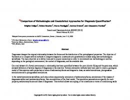
Figure-6 illustrates the performances of the detectors over an ENR range of −6 to +20 dB for − − probability of false alarm rates of and (Guo et al., 2012; Hodges, 2011).The detection curves show that the LO and SC detectors are significantly better than the GNID, whereas the LC detector exhibits the weakest performance. The ENRs of the various detection methods and the probabilities of false alarm given a of 90 percent are listed in (Table-2): Table-2. ENRs for various detection methods given a of 90 percent. ���
LO
SC
GIND
LC
0.1
5.3dB
7.27dB
7.5dB
8.1dB
0.01
8.8dB
10.8dB
10dB
12dB
As shown in (Table-2) and Figure-6, when the probability of a false alarm decreases, the performance of the GIND exceeds that of the SC detector. 4.2 Receiver Operating Characteristic (ROC) of the detectors In considering which value of � can serve as a bound in the Neyman–Pearson test (Hodges, 2011; Kay, 1998; Oppenheim and Verghese, 2010), referring to the varying curves of PD versus � as the parameter of ENR is frequently useful. Such curves are referred to as ROC curves. In general, such an ROC can be defined for any decision rule that causes PD to be uniquely fixed once PFA is specified. For instance, ROCs can be used to
3091
VOL. 11, NO. 5, MARCH 2016
ISSN 1819-6608
ARPN Journal of Engineering and Applied Sciences ©2006-2016 Asian Research Publishing Network (ARPN). All rights reserved.
www.arpnjournals.com
�
= .
Figure-6. Performance of the LO detector, SC detector, GNID, and LC detector. (a) identify whether modifying the variable parameters in a given test to permit a slightly high PFA results in a significantly highPD . ROCs can also be used to compare different tests. The ROC curve was first developed by electrical engineers and radar engineers during World War II to detect aircrafts from radar signals after an attack. Figure-7(a) shows the ROC detection curves of the detectors at a low ENR of 0 dB. The LO and SC detectors clearly display the best performances relative to the GNID. The LC detector shows the weakest performance because it is unable to achieve low false alarm probabilities. Figure-7(b) and (c) show the ROC curves at moderate ENRs of 5 and 10 dB, respectively. The same trend is clearly visible; that is, the LO and SC detectors exhibit the best performance, followed by the GNID and the LC detector. However, for high ENRs and low probabilities of false alarm, the performance of the GNID is better than that of the SC and LC detectors. 5. CONCLUSIONS UWAN in tropical shallow waters shows an accentuated impulsive behavior and thus does not follow a Gaussian distribution. The analysis of field data measurements showed that the noise amplitude distribution effectively fitted the Student’s t distribution with three degrees of freedom. The knowledge of noise statistics assisted in improving the LO detector and GIND. Both detectors performed better than the conventional LC detector, as indicated by the detection probability ) and ROC curves. For unknown noise statistics, an SC detector can be used. The performance of this detector was found to be similar but slightly inferior to that of the optimal LO detector depending on the same curves mentioned previously. The near-optimal performance and simple implementation of the SC detector make it an attractive tool for sonar and underwater digital communication.
�
= . �
= . . (b)
�� =
�
= .
.
�
�� = 5 �
3092
VOL. 11, NO. 5, MARCH 2016
ISSN 1819-6608
ARPN Journal of Engineering and Applied Sciences ©2006-2016 Asian Research Publishing Network (ARPN). All rights reserved.
www.arpnjournals.com Burrowes G. and Khan J. Y. 2011. Short-range underwater acoustic communication networks: INTECH Open Access Publisher. Chitre M., Potter J. and Heng O. S. 2004. Underwater acoustic channel characterisation for medium-range shallow water communications. Paper presented at the OCEANS'04. MTTS/IEEE TECHNO-OCEAN'04. Chitre M., Potter J. R. and Ong S.-H. 2006. Optimal and near-optimal signal detection in snapping shrimp dominated ambient noise. Oceanic Engineering, IEEE Journal of. 31(2): 497-503. �� =
�
Figure-7. ROC curves of the LO detector, SC detector, GNID, and LC detector at (a) ENR = 0 dB, (b) ENR = 5 dB, and (c) ENR = 10 dB. ACKNOWLEDGEMENTS The authors thank the Faculty of Electrical Engineering, Universiti Teknologi Malaysia (UTM) for their support and cooperation during this study. The first author would like to thanks the Ministry of Higher Education and Scientific Research, Iraq for providing Doctoral scholarship for his study. REFERENCES Abramowitz M. and Stegun I. A. 1964. Handbook of mathematical functions: with formulas, graphs, and mathematical tables: Courier Corporation. Ahsanullah M., Kibria B. G. and Shakil M. 2014. Normal and Student's T Distributions and Their Applications: Springer. Baili J., Lahouar S., Hergli M., Al-Qad, I. L. and Besbes K. 2009. GPR signal de-noising by discrete wavelet transform. NDT and E International. 42(8): 696-703. Baleanu D. 2012. Advances in wavelet theory and their applications in engineering, physics and technology. Bouvet M. and Schwartz S. C. 1986. Detection in underwater noises modeled as a Gaussian-Gaussian mixture. Paper presented at the Acoustics, Speech, and Signal Processing, IEEE International Conference on ICASSP'86. Bouvet M. and Schwartz S. C. 1989. Comparison of adaptive and robust receivers for signal detection in ambient underwater noise. Acoustics, Speech and Signal Processing, IEEE Transactions on. 37(5): 621-626.
Conover W. J. and Conover W. 1980. Practical nonparametric statistics. Donoho D. L. 1995. De-noising by soft-thresholding. Information Theory, IEEE Transactions on. 41(3): 613627. Guo G., Mandal M. and Jing Y. 2012. A robust detector of known signal in non-Gaussian noise using threshold systems. Signal Processing. 92(11): 2676-2688. Hodges R. P. 2011. Underwater acoustics: Analysis, design and performance of sonar: John Wiley and Sons. Kassam S. A. 2012. Signal detection in non-Gaussian noise: Springer Science and Business Media. Kay S. M. 1998. Fundamentals of statistical signal processing, Vol. II: Detection Theory. Signal Processing. Upper Saddle River, NJ: Prentice Hall. Lilliefors H. W. 1969. On the Kolmogorov-Smirnov test for the exponential distribution with mean unknown. Journal of the American Statistical Association. 64(325): 387-389. Liu Y., Huang Z.-p., Su S.-j. and Liu C.-w. 2012. AR model whitening and signal detection based on GLD algorithm in the non-Gaussian reverberation. Applied Acoustics. 73(10): 1045-1051. Melodia T., Kulhandjian H., Kuo L.-C. and Demirors E. 2013. Advances in underwater acoustic networking. Mobile Ad Hoc Networking: Cutting Edge Directions. pp. 804-852. Murugan S. S., Natarajan V. and Kumar R. R. 2012. Estimation of noise model and denoising of wind driven ambient noise in shallow water using the LMS algorithm. Acoustics Australia. 40(2): 111.
3093
VOL. 11, NO. 5, MARCH 2016
ISSN 1819-6608
ARPN Journal of Engineering and Applied Sciences ©2006-2016 Asian Research Publishing Network (ARPN). All rights reserved.
www.arpnjournals.com Nason G. P. 2006. On the sum of t and Gaussian random variables. Statistics & probability letters, 76(12), 12801286. Oppenheim, A. V. and Verghese, G. C. (2010). Signals, systems, and inference. Class notes for, 6. Panaro J., Lopes F., Barreira L. M. and Souza F. E. 2012. Underwater Acoustic Noise Model for Shallow Water Communications. Paper presented at the Brazilian Telecommunication Symposium. Peebles P. Z., Read J. and Read P. 2001. Probability, random variables, and random signal principles (Vol. 3): McGraw-Hill New York. Sha'ameri A. Z., Al-Aboosi Y. and Khamis N. H. H. 2014. Underwater Acoustic Noise Characteristics of Shallow Water in Tropical Seas. Paper presented at the Computer and Communication Engineering (ICCCE), 2014 International Conference on. Stojanovic M. and Preisig J. 2009. Underwater acoustic communication channels: Propagation models and statistical characterization. Communications Magazine, IEEE. 47(1): 84-89. Therrien C. W. 1992. Discrete random signals and statistical signal processing: Prentice Hall PTR. Young R. K. 2012. Wavelet theory and its applications (Vol. 189): Springer Science and Business Media.
3094