Comparison of methods to account for autocorrelation in correlation ...

Color profile: Disabled Composite Default screen

2127

Comparison of methods to account for autocorrelation in correlation analyses of fish data Brian J. Pyper and Randall M. Peterman

Abstract: Autocorrelation in fish recruitment and environmental data can complicate statistical inference in correlation analyses. To address this problem, researchers often either adjust hypothesis testing procedures (e.g., adjust degrees of freedom) to account for autocorrelation or remove the autocorrelation using prewhitening or first-differencing before analysis. However, the effectiveness of methods that adjust hypothesis testing procedures has not yet been fully explored quantitatively. We therefore compared several adjustment methods via Monte Carlo simulation and found that a modified version of these methods kept Type I error rates near α. In contrast, methods that remove autocorrelation control Type I error rates well but may in some circumstances increase Type II error rates (probability of failing to detect some environmental effect) and hence reduce statistical power, in comparison with adjusting the test procedure. Specifically, our Monte Carlo simulations show that prewhitening and especially first-differencing decrease power in the common situations where low-frequency (slowly changing) processes are important sources of covariation in fish recruitment or in environmental variables. Conversely, removing autocorrelation can increase power when lowfrequency processes account for only some of the covariation. We therefore recommend that researchers carefully consider the importance of different time scales of variability when analyzing autocorrelated data. Résumé : L’autocorrélation du recrutement des poissons et des données écologiques peut compliquer l’inférence statistique dans les analyses de corrélation. Pour régler ce problème, les chercheurs ajustent souvent les méthodes de vérification des hypothèses (p. ex. ajustement des degrés de liberté) afin de tenir compte de l’autocorrélation, ou éliminent l’autocorrélation par l’introduction de bruit blanc ou le calcul des différences premières. Toutefois, l’efficacité des méthodes servant à l’ajustement des méthodes de vérification des hypothèses n’a pas encore été entièrement étudiée sur le plan quantitatif. Nous avons donc comparé plusieurs méthodes d’ajustement par la simulation de Monte Carlo et nous avons constaté qu’une version modifiée de ces méthodes permet de maintenir le taux d’erreur de type I près de α. Par contraste, les méthodes qui éliminent l’autocorrélation contrôlent bien le taux d’erreur de type I mais dans certains cas, elles augmentent le taux d’erreur de type II (probabilité de ne pas déceler certains effets écologiques) et donc, réduisent l’efficacité statistique comparativement à l’ajustement de la méthode de vérification. Plus particulièrement, nos simulations de Monte Carlo montrent que l’introduction de bruit blanc, et surtout le calcul des différences premières, diminuent l’efficacité dans des situations ordinaires où les processus à basse fréquence (à évolution lente) sont des sources importantes de covariation du recrutement des poissons ou des variables de l’environnement. Réciproquement, l’élimination de l’autocorrélation peut accroître l’efficacité statistique lorsque les processus à basse fréquence ne représentent qu’une certaine partie de la covariation. Nous recommandons donc aux chercheurs de considérer attentivement l’importance des différentes échelles de temps de la variabilité lorsqu’ils analysent des données autocorrélées. [Traduit par la Rédaction]

Pyper and Peterman

One of the greatest challenges in fish biology and management is to understand mechanisms associated with highly variable survival rates and recruitment in fish populations. This variability can occur over various time scales or frequencies. For instance, rapid year-to-year changes (variability at higher frequencies) in fish survival rates, zooplankton Received September 19, 1997. Accepted June 23, 1998. J14211 B.J. Pyper1 and R.M. Peterman. School of Resource and Environmental Management, Simon Fraser University, Burnaby, BC V5A 1S6, Canada. 1

Author to whom all correspondence should be addressed. e-mail: [email protected]

Can. J. Fish. Aquat. Sci. 55: 2127–2140 (1998)

I:\cjfas\cjfas55\CJFAS-09\CJFAS-9C.vp Thursday, October 08, 1998 2:20:18 PM

2140

abundance, and oceanographic variables are commonly observed characteristics of marine ecosystems, where values of a given variable are largely independent from one year to the next. In recent years, however, fisheries scientists and oceanographers have found increasing evidence of slowly changing, long-term variations (variability at lower frequencies) in these biological and physical variables (e.g., Beamish 1995), such that values in a given year are closely related to values in previous years (i.e., the data contain positive autocorrelation). This longer term variability has been exhibited in the Northeast Pacific Ocean, for example, by extended periods of unusually high sea-surface temperatures, weak upwelling, and low biological productivity followed by periods of the opposite. Correlation analysis has been a useful and widely applied tool for generating hypotheses about the effects of environ© 1998 NRC Canada

Color profile: Disabled Composite Default screen

2128

mental or other variables on recruitment at these various time scales (e.g., Myers et al. 1995a, and papers cited therein). However, a major statistical challenge exists when time series of recruitment and environmental data are strongly autocorrelated, i.e., dominated by low-frequency variability (e.g., Chelton 1984; Thompson and Page 1989). Such autocorrelation violates the assumption of serial independence required for most classical inference tests (Hurlbert 1984). In general, this means that a sample correlation between two autocorrelated time series has fewer degrees of freedom (or a larger variance) than that assumed under the classical significance test. Consequently, the test will have a Type I error rate greater than the specified α (i.e., there will be an increased chance of concluding that a correlation is statistically significant when in fact no correlation is present; Jenkins and Watts 1968, p. 338). To address this problem, fisheries scientists and oceanographers have typically applied two qualitatively different approaches. One approach is to modify the hypothesis testing procedure by computing either a corrected degrees of freedom for the sample correlation (Garrett and Petrie 1981; Chelton 1984) or, equivalently, a corrected variance for the sample correlation (Kope and Botsford 1990). The usefulness of these methods has been questioned, however, because they depend on the autocorrelation function of each time series, which can be poorly estimated for short time series typical of fisheries data sets (Thompson and Page 1989). Despite the importance of this statistical problem, we are not aware of any publications examining the ability of these methods to control Type I error rates. This paper therefore attempts to fill this gap. The second approach to dealing with autocorrelation attempts to remove it from each time series of data before computing and testing correlations. This has been done either by fitting time series models to the data and using residuals from them (often referred to as “prewhitening”; e.g., Milicich et al. 1992; Quinn and Niebauer 1995) or by “firstdifferencing” the data (subtracting each data point from the next; e.g., Thompson and Page 1989). The premise behind these methods is that if the new transformed data series are free of autocorrelation, then classical inference tests are appropriate for correlations computed between them. However, because removing autocorrelation is equivalent to removing low-frequency variability from data, a potential drawback of prewhitening and first-differencing seems clear: if the lowfrequency components of variability in two time series of recruitment or environmental data are common (i.e., synchronous or asynchronous), as some researchers are finding (see Beamish 1995), then removing autocorrelation may also remove much of this covariance (Thompson and Page 1989). Such procedures may thus increase the probability that researchers will miss finding some important relationship between long-term, slowly changing environmental processes and fish population dynamics. In other words, they may face an increased Type II error rate (i.e., probability of failing to reject the null hypothesis of no correlation when it is in fact false). In many of the papers we reviewed, however, the researchers did not seem to recognize this potential drawback of removing autocorrelation. This paper has two main objectives. First, we use Monte Carlo simulations to examine the effectiveness of several

Can. J. Fish. Aquat. Sci. Vol. 55, 1998

commonly employed methods for adjusting the test procedure of the null hypothesis of no correlation between autocorrelated data (Garrett and Petrie 1981; Chelton 1984; Kope and Botsford 1990). Specifically, we examine how closely the Type I error rates of these methods match the specified α. Second, we use a simple model and Monte Carlo simulations to illustrate the degree to which prewhitening and first-differencing can alter levels of real covariation between autocorrelated data and affect Type II error rates in comparison with the best method for adjusting the test procedure. For completeness, we also examine how levels of covariation and Type II error can be altered by “smoothing” data, a method that, in contrast with prewhitening and first-differencing, is frequently used to remove high-frequency components of variability from data. In addition, we provide an empirical example using recruitment data for several stocks of sockeye salmon (Oncorhynchus nerka) from Bristol Bay, Alaska. We limit our analyses of Type I and Type II error rates to the case where correlations are being computed at a single lag, which is typical of most fisheries applications. Furthermore, because our main intended audience is fisheries biologists, all methods and results are in the context of the time domain (i.e., correlations and autocorrelations), rather than the frequency domain often used by oceanographers (i.e., spectral analysis).

Garrett and Petrie (1981), Chelton (1984), and Kope and Botsford (1990) provide similar methods for adjusting the null hypothesis test of a sample correlation between two autocorrelated time series, say X and Y. These methods, which are based on formulas from either Bayley and Hammersley (1946) or Bartlett (1946), assume that the time series are stationary, such that their underlying means remain constant over time. Furthermore, when testing a sample correlation at a given lag k, denoted rXY(k), each of these methods assumes a null hypothesis of no correlation at all lags. These methods can be summarized using the following theoretical approximation of the “effective” number of degrees of freedom, N*, of rXY (k) (1)

1 1 2 ≈ + N N N*

∞

(N − j) ρ XX ( j )ρYY ( j ) N j =1

∑

where N is the sample size and ρXX (j) and ρYY (j) are the autocorrelations of X and Y at lag j. For example, Garrett and Petrie (1981) used a form of eq. 1 where ρXX (j)ρYY (j) was replaced by ρ(j), the autocorrelation at lag j of the crossproduct of X and Y (each standardized to have a mean of zero). Given N*, Garrett and Petrie (1981) used the standard critical value for rXY(k) at the α significance level that can be read from statistical tables or derived using the t distribution for either one- or two-tailed tests (Zar 1984, p. 309): (2)

rcrit =

t α2 , N * (t α2 , N * + N * ). © 1998 NRC Canada

I:\cjfas\cjfas55\CJFAS-09\CJFAS-9C.vp Thursday, October 08, 1998 2:20:19 PM

Color profile: Disabled Composite Default screen

Pyper and Peterman

Chelton (1984) recommended an expression for N* that is equivalent to eq. 1 but without the weighting function (N − j)/N. Chelton also recommended an alternative critical value based on the chi-square distribution with 1 degree of freedom, which is equivalent to the following, based on the standard normal distribution (Z): (3)

rcrit = Z α 2 1 N *

where values of α and α/2 are used for one- and two-tailed tests, respectively. Kope and Botsford (1990) provided an approximation for the variance of a sample correlation that is equivalent to 1/N* as defined by eq. 1. They assumed that the null distribution of rXY(k) is normal, which also implies the critical value defined by eq. 3. Thus, the only difference between their method and that of Chelton is that Kope and Botsford included the weighting function (N – j)/N in the computation of N* (eq. 1). Each of the above methods for adjusting the test procedure attempts to maintain Type I error rates at the specified α by generating critical values that account for autocorrelation. When both time series contain positive autocorrelation, it is clear from eq. 1 that values of N* will be less than N, resulting in larger, and hence more conservative, critical values (i.e., fewer rejections of the null hypothesis of no correlation than if no adjustment were made). However, these methods may perform poorly in practice for a number of reasons: (i) the expressions for N* are based on asymptotic (large sample size) formulas that may not be accurate for short time series, (ii) values of N* depend on estimates of autocorrelation functions that are known to be both imprecise and biased, especially for short time series (Jenkins and Watts 1968, chap. 5), and (iii) the distributions assumed by critical values (2) and (3) may be inappropriate, particularly for short time series with high levels of autocorrelation. In addition, it is unclear how many lags j should be used when computing N*. Given these potential problems, we conducted the following simulation analysis to examine the performance of these methods. Methods—adjusting the test procedure We used simple time series models to generate hypothetical data sets with lengths (number of years) and levels of positive autocorrelation that were typical of recruitment and environmental time series. Recruitment series used in correlation analyses often vary from about 15 years to usually not more than 50 years (e.g., Myers et al. 1995a), and it is common to observe estimates of lag-1 autocorrelation ranging from moderate (e.g., 0.5) to high values (e.g., 0.8) (e.g., Koslow et al. 1987). In our baseline analysis, we simulated two independent time series X and Y of length N using first-order autoregressive models (AR(1) models) (Box and Jenkins 1976, p. 56): (4)

X t = φX X t −1 + εt

and similarly for Y, where ε was randomly and normally distributed and φX is the autoregressive parameter. The variance of X as defined by eq. 4 is σ2X = σ2ε ( 1 − φX2 ), which was used

2129

to generate the initial value of X. Note that X has a theoretical autocorrelation function (5)

ρ XX ( j) = φ|Xj |

such that greater absolute values of φX give rise to more autocorrelated time series. Also note that the value of φX corresponds to the theoretical lag-1 autocorrelation in the time series. AR(1) models can produce a wide range of autocorrelated time series and often provide a reasonable description of fisheries and ecological data. We generated X and Y with N ranging from 15 to 50 years (in increments of 5) and with the same autoregressive parameter φ (i.e., φX = φY) ranging from 0.4 to 0.9 (in increments of 0.1). For each combination of N and φ, 5000 Monte Carlo trials were done in which we computed sample correlations between the two time series at lag zero (i.e., using the N pairs of simulated data) and tabulated Type I error rates for two-tailed tests of the null hypothesis of no correlation for three levels of α (0.02, 0.05, and 0.10) using the following testing methods: (A) the standard significance test using critical value (2) and N – 2 degrees of freedom (i.e., not making any adjustments for autocorrelation), (B) the Garrett–Petrie method, (C) the Chelton method, and (D) the Kope–Botsford method. For methods B–D, autocorrelations were estimated over the first N/4 lags (i.e., j = 1 to N/4 in eq. 1) using an estimator recommended by Box and Jenkins (1976, p. 32): N−j

(6)

rXX ( j ) =

∑ (X t − X )(X t+ j − X ) t =1

N

.

∑ (X t − X )2 t =1

On occasion, variability in autocorrelation estimates resulted in values of N* that were greater than the sample size N. We followed Kope and Botsford (1990) and constrained N* to a maximum of N. We examined the sensitivity of the methods to the choice of critical value, autocorrelation estimator, the number of lags for which autocorrelations were estimated, and the type of time series model used in the simulations. Results and discussion—adjusting the test procedure A summary of Type I error rates is shown in Table 1 for each of the methods A–D described above. Results for the standard significance test provide a baseline for comparison (Table 1, Case A). In this case, error rates were consistently much greater than the specified α values and increased rapidly as φ increased, as illustrated in Fig. 1A for α = 0.05. This bias emphasizes the importance of accounting for autocorrelation. However, the efficacy of the methods designed to control Type I error rates varied considerably. The Garrett–Petrie method performed poorly at the three α values (Case B), with error rates larger than α and increasing with φ (e.g., Fig. 1B). In contrast, the Chelton and Kope– Botsford methods gave very similar error rates (Cases C and D) that were somewhat conservative at α = 0.02, reasonably accurate although variable at α = 0.05, but greater and more variable than desired at α = 0.10. Error rates of these two © 1998 NRC Canada

I:\cjfas\cjfas55\CJFAS-09\CJFAS-9C.vp Thursday, October 08, 1998 2:20:20 PM

2130

Type I error rates α = 0.02

Hypothesis test procedure Case

Time series model

Method

A B C D E F G H J K L M N P Q R S T U

AR(1)a AR(1)a AR(1)a AR(1)a AR(1)a AR(1)a AR(1)a AR(1)a AR(1)a AR(1)a AR(1)a AR(1)a AR(2)b AR(2)b AR(2)c AR(2)c ARIMA(1,1,0)d ARIMA(1,1,0)d ARIMA(1,1,0)e

Standard significance test Garrett–Petrie Chelton Kope–Botsford Chelton using theoretical N* Chelton; theoretical N*; critical value (2) Chelton using critical value (2) Modified Chelton Modified Chelton with eq. 7 Modified Chelton with eq. 7 Modified Chelton with eq. 7 Modified Chelton with eq. 7 Standard significance test Modified Chelton with eq. 7 Standard significance test Modified Chelton with eq. 7 Standard significance test Modified Chelton with eq. 7 Modified Chelton with eq. 7

No. of lags j N/4 N/4 N/4

N/4 N/4 N/4 N/3 N/5 N/6 N/5 N/5 N/5 N/5

α = 0.05

α = 0.10

Average

Range

Average

Range

Average

Range

0.143 0.095 0.013 0.015 0.006 0.013 0.031 0.018 0.014 0.012 0.016 0.017 0.141 0.016 0.118 0.011 0.593 0.016 0.047

0.034–0.389 0.027–0.215 0.007–0.017 0.008–0.018 0.000–0.016 0.000–0.023 0.019–0.066 0.013–0.022 0.011–0.017 0.009–0.015 0.011–0.018 0.012–0.021 0.026–0.384 0.011–0.021 0.078–0.358 0.005–0.021 0.303–0.768 0.011–0.021 0.033–0.063

0.212 0.154 0.056 0.062 0.024 0.037 0.081 0.053 0.044 0.038 0.047 0.049 0.212 0.049 0.265 0.035 0.654 0.055 0.114

0.080–0.474 0.063–0.299 0.041–0.078 0.043–0.098 0.000–0.047 0.001–0.058 0.051–0.168 0.043–0.069 0.037–0.047 0.032–0.044 0.043–0.051 0.044–0.057 0.064–0.469 0.040–0.058 0.140–0.436 0.021–0.061 0.395–0.808 0.050–0.062 0.081–0.155

0.29 0.23 0.14 0.15 0.07 0.08 0.16 0.12 0.10 0.09 0.11 0.11 0.29 0.11 0.35 0.08 0.71 0.14 0.22

0.15–0.55 0.12–0.39 0.10–0.23 0.10–0.25 0.00–0.10 0.01–0.12 0.11–0.28 0.09–0.16 0.09–0.12 0.08–0.10 0.09–0.12 0.09–0.14 0.13–0.55 0.09–0.14 0.22–0.52 0.06–0.13 0.48–0.84 0.13–0.15 0.17–0.28

Note: The average and range of each set of simulations were computed across all combinations of N (ranging from 15 to 50 in increments of 5) and the parameter values of the time series model. See text for details. a Parameter range for φ: 0.4 to 0.9 (increments of 0.1). b Parameter range for φ1: 0.2 to 0.7 (increments of 0.1); φ2: 0.2 to (0.9 – φ1) (increments of 0.1). c Parameter range for φ1: 0.8 to 1.8 (increments of 0.2); φ2: – φ1/2. d Parameter range for φ: 0.0 to 0.6 (increments of 0.3). e Parameter value for φ: 0.9.

Color profile: Disabled Composite Default screen

I:\cjfas\cjfas55\CJFAS-09\CJFAS-9C.vp Thursday, October 08, 1998 2:20:22 PM

Table 1. Summary of simulated Type I error rates for different methods of adjusting the hypothesis test procedure, different time series models, and three levels of α.

Can. J. Fish. Aquat. Sci. Vol. 55, 1998

© 1998 NRC Canada

Color profile: Disabled Composite Default screen

Pyper and Peterman

2131

Fig. 1. Isopleths of simulated Type I error rates at α = 0.05 for (A) the standard inference test, (B) the Garrett–Petrie method, (C) the Chelton method, (D) the Chelton method using theoretical values of N*, (E) the Chelton method using critical value (2) instead of critical value (3), and (F) the Modified Chelton method (i.e., using critical value (2) with N* – 2). See text for details.

methods also increased as φ increased, especially for small N (e.g., Fig. 1C). The Garrett–Petrie method was not as effective as the Chelton and Kope–Botsford methods primarily because estimates of ρ(j), the autocorrelation function of the crossproduct used in eq. 1, were highly imprecise and often negative for lags greater than 1 or 2, resulting in large overestimates of N*. Changing the number of lags j used to estimate N* did little to improve performance. For long time series (e.g., N = 1000), we found that estimates of ρ(j) were very similar to those of ρXX (j)ρYY (j) (the product used in the Chelton and Kope–Botsford methods), but for short time series, ρ(j) was consistently smaller and much more variable. We therefore recommend that researchers not use the Garrett–Petrie approach. For a given α value, Type I error rates of the Kope–

Botsford method (Table 1, Case D) were slightly larger and more variable than those of the Chelton method (Case C). Recall that the only difference between these methods is that the Kope–Botsford method includes the weighting function (N – j)/N in eq. 1. This added weighting function produced slightly larger estimates of N*, which, over the various simulations we performed, consistently resulted in error rates that were slightly more variable than those of the Chelton method. We therefore limit further discussions of results to the Chelton method. We found that the Type I error rates of the Chelton method were largely determined by an interaction among three main factors. First, it appears that eq. 1 (with or without the weighting function) does not provide accurate “theoretical” values of N* for short, autocorrelated time series. For example, we used the theoretical autocorrelation func© 1998 NRC Canada

I:\cjfas\cjfas55\CJFAS-09\CJFAS-9C.vp Thursday, October 08, 1998 2:20:28 PM

Color profile: Disabled Composite Default screen

2132 Fig. 2. Isopleths of (A) theoretical values of N* computed using the theoretical autocorrelation functions of X and Y (eq. 5) and Chelton’s form of eq. 1 and (B) average simulated estimates of N* computed using Chelton’s form of eq. 1.

tions of X and Y (eq. 5) and Chelton’s form of eq. 1 to compute the theoretical N* for each combination of N and φ (Fig. 2A). However, when these values of N* were used with critical value (3), error rates were typically much too conservative (Table 1, Case E), falling well below the specified α values as φ increased (e.g., Fig. 1D). Results were similar for critical value (2) (Case F). Second, estimates of autocorrelation were biased low in our simulations (i.e., toward less positive values), resulting in estimates of N* that were considerably larger than the theoretical values of N* (Fig. 2). Changing the number of lags j used to estimate N* did little to reduce these differences. Standard estimators of autocorrelation can be seriously biased in this direction, with biases increasing for shorter time series or larger autocorrelations (e.g., Marriott and Pope 1954). Consequently, these biases compensated somewhat for the fact that theoretical values of N* are overly conservative at high φ (e.g., Fig. 1D), resulting in error rates for the Chelton method that were reasonably accurate for α = 0.05 (Fig. 1C). Third, critical value (3) (based on the normal assumption) is inappropriate for autocorrelated data when N is small, just as it would be for the standard case where data are serially independent and critical value (2) is appropriate (Zar 1984, p. 309). When N is small (e.g., φI). For example, Table 2 presents asymptotic correlations for four combinations of φI and φC when (a, b, σI X , σIY , σC ) = 1. For the extreme case where φI = 0 and φC = 0.9, prewhitening and firstdifferencing will reduce ρXY from 0.50 to only 0.25 and 0.09, respectively. In contrast, smoothing will increase ρXY from 0.50 to 0.66. However, when independent sources of variability are the primary sources of autocorrelation (φI > φC), prewhitening and first-differencing will increase ρXY, while smoothing reduces it (right side of Table 2). In the case where φC > φI, it is conceivable that reductions in correlations caused by prewhitening or first-differencing may be offset by the increase in degrees of freedom obtained by removing autocorrelation, which could increase or at least maintain statistical power. However, our simulations showed that in many cases, statistical power was reduced substantially. Figure 4 presents isopleths of changes in statistical power for three combinations of N and (a,b) when X and Y were either prewhitened, first-differenced, or smoothed. Positive values indicate increases in statistical power, while negative values (shaded areas in Fig. 4) indicate decreases. For example, a value of –0.2 means that out of 100 tests, there would be 20 fewer cases in which the null hypothesis was correctly rejected compared with using the © 1998 NRC Canada

I:\cjfas\cjfas55\CJFAS-09\CJFAS-9C.vp Thursday, October 08, 1998 2:20:37 PM

Color profile: Disabled Composite Default screen

2136

Can. J. Fish. Aquat. Sci. Vol. 55, 1998

Table 2. Theoretical asymptotic correlations, computed from equations in Table A (see Appendix), between time series X and Y for the original time series, prewhitened series, firstdifferenced series, and smoothed series. Asymptotic correlation between X and Y (ρXY) Transformation of data (A) (B) (C) (D)

Original Prewhitened First-differenced Smoothed

φI = 0.0

φC = 0.0

φC = 0.6

φC = 0.9

φI = 0.6

φI = 0.9

0.50 0.40 0.29 0.62

0.50 0.25 0.09 0.66

0.50 0.60 0.71 0.38

0.50 0.75 0.91 0.34

Note: ( a , b, σ I X , σ I Y , σ C ) = 1 and φ I X = φ I Y = φ I .

original time series and the Modified Chelton test procedure. (Note that eqs. A1 and A3 in the Appendix provide a rough indication of the levels of covariation and autocorrelation in the original time series X and Y for given values of (a,b), φI, and φC.) For small values of (a,b) (i.e., small effect of the common factor C), prewhitening and first-differencing increased statistical power in most cases, especially for φI >> φC (e.g., N = 20 and (a,b) = 0.6; top panels in Fig. 4). However, the situation changed appreciably when the common factor was a more important source of variability in X and Y (e.g., N = 20 and (a,b) = 1.4; middle panels in Fig. 4). Here, prewhitening and first-differencing resulted in reductions in power by as much as 0.2 or 0.3 for combinations where φC > φI and resulted in increases in power that were greatest when both φI and φC were large. Larger changes in power were observed for given values of (a,b) when N = 50 (e.g., N = 50 and (a,b) = 1.0; bottom panels in Fig. 4). The patterns shown in Fig. 4 for prewhitening and firstdifferencing were typical of the range of combinations of N and (a,b) that we explored. In general, these transformations increased power when φI > φC by increasing degrees of freedom and levels of covariation. However, when φC > φI, removing autocorrelation typically reduced power despite increasing degrees of freedom because these procedures resulted in often large reductions in covariation. Interestingly, smoothing using a two-point running mean increased power only slightly when φC >> φI (Fig. 4). For most combinations where φC > φI, increases in covariation due to smoothing were offset by decreased degrees of freedom (through increased autocorrelation), resulting in reduced power. Using three-, four-, or five-point running means also resulted in only slight increases in power when φC >> φI. Thus, as illustrated by this theoretical example, prewhitening and, in particular, first-differencing can remove much of the covariation between autocorrelated time series and consequently reduce the power to detect it when the source of that covariation is also the main source of the autocorrelation. Of course, the opposite is also true. That is, if autocorrelation is due in large part to variability that is unique to a given time series, then prewhitening or firstdifferencing can substantially increase power. It is not our purpose to present an exhaustive examination of the advantages or disadvantages of such methods as prewhitening, first-differencing, or smoothing, but rather to point out that

such transformations may have unintended effects that alter the interpretation of analyses. By using prewhitening or first-differencing, past researchers may have missed detecting some environmental effect or some correlation among stocks that existed due to the common effect of some important but slowly changing variable. A final frequently used method of treating time series in fisheries is to remove time trends. Recruitment and environmental time series often have distinct increasing or decreasing trends over time (e.g., Cohen et al. 1991) that could easily produce misleading correlations between the series when these trends are independent (Plosser and Schwert 1978) or could mask covariation at higher frequencies (Kope and Botsford 1990). Furthermore, strong trends indicate nonstationary time series, in which case, methods for adjusting the test procedure may not adequately control type I error rates. Thus, some researchers recommend removing time trends before computing correlations by either firstdifferencing (e.g., Cohen et al. 1991) or “detrending” the data (typically using residuals from a linear regression versus time) (e.g., Botsford and Brittnacher 1992). Once again, however, such practices may remove important information about a possible common mechanism influencing different data series. By removing time trends, we are assuming that they are unrelated, yet there are obvious mechanisms that could produce common time trends among recruitment data such as trends in environmental variables, habitat degradation, or trends in the abundances of competitor, prey, or predator species (e.g., Butler 1991). In addition, short time series can often appear to have deterministic or nonstationary trends, even though the series are stationary and only moderately autocorrelated. Thus, even though we may not be able to distinguish between time trends that are caused by a common mechanism and those that are not, researchers should consider both possibilities when choosing methods of analysis and they should interpret their results cautiously.

The previous section quantified potential changes in correlations and statistical power that could be caused by prewhitening, first-differencing, and smoothing. Here, we briefly illustrate the possible effects of these transformations using recruitment data for four stocks of sockeye salmon from Bristol Bay, Alaska. There has been growing interest in the low-frequency variability, often referred to as interdecadal variability, of physical and biological processes in the North Pacific and their effects on the productivity of fish stocks such as Bristol Bay sockeye (e.g., Hare and Francis 1995; Adkison et al. 1996). Methods—empirical example We selected four stocks of Bristol Bay sockeye that had autocorrelated indices of survival rate: the Igushik, Kvichak, Ugashik, and Wood River stocks. For each stock, we used abundances of spawners and total recruits for 34 brood years from 1956 to 1989 (B. Cross, Alaska Department of Fish and Game, Anchorage, Alaska, personal communication). Using these data, we computed an index of survival rate (SR © 1998 NRC Canada

I:\cjfas\cjfas55\CJFAS-09\CJFAS-9C.vp Thursday, October 08, 1998 2:20:38 PM

Color profile: Disabled Composite Default screen

Pyper and Peterman

2137

Fig. 4. Isopleths of changes in statistical power for prewhitening, first-differencing, and smoothing compared with using the original time series and the Modified Chelton method for three sets of conditions of N and (a,b). Positive values indicate increases in statistical power over using the original time series, while negative values indicate decreases. See text for details. 0.3 0.2 0.1

(a,b) = 0.6

-0.1

0.3 0.2 0.1

0.0

0.9

-0.2

0.4

N = 20

Smoothed

0.6 -0.05

0.0

0.3

0.0 0.0

0.0

0.05 0.0

0.9 0.2

0.1

0.2

N = 20

-0.25 0.1

(a,b) = 1.4 0.0

0.0 -0.1 -0.2

0.1

N = 50

0.2

0.3 0.1

-0.2

0.6 -0.15 -0.1

-0.1 -0.2

0.2

-0.05

-0.3

0.3

0.0

0.3 -0.3

0.6

-0.2

(a,b) = 1.0 0.0

0.0 -0.1

0.0

0.3

0.6

-0.1 -0.1 -0.3

-0.2

0.9

0.3 0.0 0.1

-0.5

0.0

0.3

0.6

φC (autocorrelation in the common variable)

index) for each stock to account for changes in spawner abundance, within-stock density dependence, and lognormal error structure. This index was the time series of residuals from the fit of the Ricker stock–recruitment relationship, i.e., linear regression of loge(recruits per spawner) versus spawners. The autocorrelation and partial autocorrelation functions of the four SR indices were consistent with AR(1) processes, with estimates of lag-1 autocorrelation ranging from 0.44 to 0.70. We therefore fit AR(1) models to these SR indices as an example of prewhitening. We computed pairwise correlations among the four SR data series using the original, prewhitened, first-differenced, and smoothed data (two-point running mean). Standard hypothesis tests (two-tailed, α = 0.05) were used for correlations among prewhitened or first-differenced data, while the Modified Chelton method was used for correlations among the original or smoothed data. Statistical power was estimated for each pairwise comparison using the sample correlation and the equations given in Zar (1984, p. 312). Because these “analytical” equations are for serially independent data, they provide only a rough approximation of power for comparisons among the original and smoothed (i.e., autocorrelated) data. However, in our simulation analyses described above, we found that the analytical estimates of power consistently underestimated the actual, simulated power by roughly 0.05 on average for cases where levels of covariation and autocorrelation were similar to those ob-

0.0 0.9

(autocorrelation in the independent variables)

First-Differenced

φI

Prewhitened

0.0 0.9

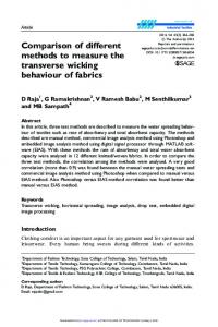
served here for the four Bristol Bay sockeye stocks. Thus, the estimates of power provided below for the original and smoothed data are likely slight underestimates of the actual statistical power. Results and discussion—empirical example The time series of SR indices and their transformations are shown in Fig. 5. Extended periods of negative residuals (1960s) and positive residuals (1970s) in each of the original SR indices provide evidence that synchronous lowfrequency variability is an important feature of these data (Fig. 5A), suggesting a shared influence of some autocorrelated environmental factor. Prewhitening and, in particular, first-differencing appeared to remove much of the coherence between the SR indices (Figs. 5B and 5C). In contrast, using a two-point running mean to smooth the SR indices accentuated the low-frequency trends and the apparent coherence of the time series (Fig. 5D). Correlations among the original and transformed SR indices (Table 3) reflect the patterns observed in Fig. 5. For example, prewhitening and first-differencing reduced the average correlation among the SR series from 0.50 to only 0.24 and 0.11, respectively (last row of Table 3), and reduced the number of significant correlations from 4 to 2 and 1, respectively. Moreover, prewhitening and, to a greater extent, first-differencing reduced the average statistical power from 0.5 to 0.34 and 0.18, respectively, despite having twice © 1998 NRC Canada

I:\cjfas\cjfas55\CJFAS-09\CJFAS-9C.vp Thursday, October 08, 1998 2:20:43 PM

Color profile: Disabled Composite Default screen

0.51 0.18 0.34 0.50 0.62

0.64 0.35 0.53 0.38 0.43 0.72 0.44 0.02 0.12 0.01 0.51 0.01

First-differenced Prewhitened

0.70 0.08 0.36 0.04 0.73 0.14 0.65 0.31 0.58 0.32 0.60 0.56

Original Smoothed

0.73* 0.52 0.68* 0.43 0.59 0.76* 0.32 –0.02 0.14 –0.10 0.35* –0.06

First-differenced

0.11 0.24 0.50 9 14

Note: *Statistically significant (P < 0.05).

A growing body of literature documents the importance of slow changes, or low-frequency variability, in recruitment of fish species and in the physical and biological processes that

Average

the number of degrees of freedom as the average comparison among the original, autocorrelated SR indices (i.e., 31 versus an average of 14 degrees of freedom) (right half of Table 3). In contrast, smoothing increased the average correlation to 0.62, although statistical power changed little because of the corresponding decreases in degrees of freedom (Table 3). Thus, this example represents a case where the researcher could easily miss detecting the shared influence of a slowly changing process on fish productivity by removing autocorrelation rather than adjusting the test procedure to account for autocorrelation. The tendency for correlations to be lower among prewhitened or first-differenced data and higher among smoothed data suggests that low-frequency components of variability were the dominant source of covariation in the original SR indices.

0.43* 0.11 0.28 0.05 0.44* 0.16

Smoothed Residuals

Residual

(D)

Prewhitened

First-Differenced Residuals

Residual

(C)

0.62* 0.41 0.55* 0.33 0.51* 0.56*

Prewhitened Residuals

Residual

(B)

Original

1989

7 9 7 13 8 7

1985

Smoothed

1981

11 13 13 21 16 12

1977

Original

1973

Brood Year

IGU vs. KVI IGU vs. UGA IGU vs. WOO KVI vs. UGA KVI vs. WOO UGA vs. WOO

1969

(1) (2) (3) (4) (5) (6)

1965

Comparison

1961

Statistical power

1957

Sample correlation coefficient

Residuals from Ricker Stock-Recruitment Curve

Residual

(A)

Effective degrees of freedom (N* – 2)

Fig. 5. Time series for four Bristol Bay sockeye stocks of (A) residuals from the Ricker stock–recruitment curve (i.e., survival rate (SR) indices), (B) prewhitened SR indices, (C) firstdifferenced SR indices, and (D) smoothed SR indices.

Smoothed

Can. J. Fish. Aquat. Sci. Vol. 55, 1998

Table 3. Sample correlations and corresponding statistical power for comparisons among the survival rate (SR) indices of four Bristol Bay sockeye stocks: Igushik (IGU), Kvichak (KVI), Ugashik (UGA), and Wood (WOO).

2138

© 1998 NRC Canada

I:\cjfas\cjfas55\CJFAS-09\CJFAS-9C.vp Thursday, October 08, 1998 2:20:45 PM

Color profile: Disabled Composite Default screen

Pyper and Peterman

may affect recruitment (e.g., Hollowed and Wooster 1992). However, in an increasing number of applications in fisheries and ecological literature, autocorrelation (low-frequency variability) is removed from time series before correlation analyses are conducted in an effort to control Type I error rates (e.g., Milicich et al. 1992; Meekan et al. 1993; Robertson et al. 1993). We have shown that a specific method for adjusting the test procedure of a sample correlation may often provide a useful alternative to removing autocorrelation. Our theoretical and empirical examples showed that statistical power can be significantly greater for this adjustment method in comparison with removing autocorrelation when low-frequency variability is the major source of covariation, as many researchers are finding (e.g., Beamish 1995). It is therefore important that fisheries researchers, when dealing with autocorrelated data, generate hypotheses about what time scales of variability in environmental processes are important. Given such hypotheses, researchers can then select appropriate tools for investigating patterns of covariation at these different time scales (e.g., Hollowed et al. 1987). For example, if high-frequency (i.e., rapid time scale) components of variability are the dominant source of covariation, then prewhitening (or first-differencing) may be useful because it should increase covariation and the statistical power to detect it by removing independent, lowfrequency variability that obscures the detection of that covariation. Conversely, smoothing of some form may be useful for detecting low-frequency (slow time scale) sources of covariation, although correlations must be tested using the adjustment method outlined above to account for autocorrelation that will be present in the smoothed data. In any of these cases, researchers should be aware and cautious of the distorting effects that these various transformations can have on data. While the concerns we have raised in this paper relate to simple correlation analysis, autocorrelation has similar implications for many other statistical methods such as regression (e.g., Bence 1995).

We thank Bev Cross for the Bristol Bay sockeye salmon data as well as the numerous biologists and technicians in the Alaska Department of Fish and Game who gathered the lengthy time series of data analyzed here. We thank Terrance Quinn II and Louis Botsford for useful suggestions on the draft manuscript and James R. Bence and an anonymous reviewer for their very useful comments. Funding was provided by grants to R.M. Peterman from the Ocean Production Enhancement Network (one of Canada’s Networks of Centres of Excellence) and the Natural Sciences and Engineering Research Council of Canada.

Adkison, M.D., Peterman, R.M., Lapointe, M.F., Gillis, D.M., and Korman, J. 1996. Alternative models of climate effects on sockeye salmon, Oncorhynchus nerka, productivity in Bristol Bay, Alaska, and the Fraser River, British Columbia. Fish. Oceanogr. 5: 137–152.

2139 Bartlett, M.S. 1946. On the theoretical specification and sampling properties of autocorrelated time series. J. R. Stat. Soc. Ser. B (Methodol.), 8: 27–41. Bayley, G.V., and Hammersley, J.M. 1946. The “effective” number of independent observations in an autocorrelated time series. J. R. Stat. Soc. Ser. B (Methodol.), 8: 184–197. Beamish, R.J. (Editor). 1995. Climatic change and northern fish populations. Can. Spec. Publ. Fish. Aquat. Sci. No. 121. Bence, J.R. 1995. Analysis of short time series: correcting for autocorrelation. Ecology, 76: 628–639. Botsford, L.W., and Brittnacher, J.G. 1992. Detection of environmental influence on wildlife: California quail as an example. In Wildlife 2001: populations. Edited by D.R. McCullough and R.H. Barrett. Elsevier Science, New York. pp. 158–169. Box, G.E.P., and Jenkins, G.W. 1976. Time series analysis: forecasting and control. Revised ed. Holden-Day, San Francisco, Calif. Butler, J.L. 1991. Mortality and recruitment of Pacific sardine, Sardinops sagax caerulea, larvae in the California Current. Can. J. Fish. Aquat. Sci. 48: 1713–1723. Chatfield, C. 1989. The analysis of time series: an introduction. 4th ed. Chapman and Hall, London, U.K. Chelton, D.B. 1984. Commentary: short-term climatic variability in the Northeast Pacific Ocean. In The influence of ocean conditions on the production of salmonids in the North Pacific. Edited by W. Pearcy. Oregon State University Press, Corvallis, Oreg. pp. 87–99. Cohen, E.B., Mountain, D.G., and O’Boyle, R. 1991. Local-scale versus large-scale factors affecting recruitment. Can. J. Fish. Aquat. Sci. 48: 1003–1006. Davis, R.E. 1977. Techniques for statistical analysis and prediction of geophysical fluid systems. Geophys. Astrophys. Fluid Dyn. 8: 245–277. Drinkwater, K.F., and Myers, R.A. 1987. Testing predictions of marine fish and shellfish landings from environmental variables. Can. J. Fish. Aquat. Sci. 44: 1568–1573. Garrett, C., and Petrie, B. 1981. Dynamical aspects of the flow through the Strait of Belle Isle. J. Phys. Oceanogr. 11: 376–393. Hare, S.R., and Francis, R.C. 1995. Climate change and salmon production in the northeast Pacific Ocean. In Climatic change and northern fish populations. Edited by R.J. Beamish. Can. Spec. Publ. Fish. Aquat. Sci. No. 121. pp. 357–372. Hollowed, A.B., and Wooster, W.S. 1992. Variability of winter ocean conditions and strong year classes of Northeast Pacific groundfish. ICES Mar. Sci. Symp. 195: 433–444. Hollowed, A.B., Bailey, K.M., and Wooster, W.S. 1987. Patterns in recruitment of marine fishes in the northeast Pacific Ocean. Biol. Oceanogr. 5: 99–131. Hurlbert, S.H. 1984. Pseudoreplication and the design of ecological field experiments. Ecol. Monogr. 54: 187–211. Jenkins, G.M., and Watts, D.G. 1968. Spectral analysis and its applications. Holden-Day, San Francisco, Calif. Kalbfleisch, J.G. 1985. Probability and statistical inference 1: probability. 2nd ed. Springer-Verlag, New York. Kope, R.G., and Botsford, L.W. 1990. Determination of factors affecting recruitment of chinook salmon, Oncorhynchus tshawytscha, in central California. Fish. Bull. U.S. 88: 257–269. Koslow, J.A., Thompson, K.R., and Silvert, W. 1987. Recruitment to northwest Atlantic cod (Gadus morhua) and haddock (Melanogrammus aeglefinus) stocks: influence of stock size and environment. Can J. Fish. Aquat. Sci. 44: 26–39. Marriott, F.H.C., and Pope, J.A. 1954. Bias in the estimation of autocorrelations. Biometrika, 41: 390–402. © 1998 NRC Canada

I:\cjfas\cjfas55\CJFAS-09\CJFAS-9C.vp Thursday, October 08, 1998 2:20:46 PM

Color profile: Disabled Composite Default screen

2140

Can. J. Fish. Aquat. Sci. Vol. 55, 1998

Meekan, M.G., Milicich, M.J., and Doherty, P.J. 1993. Larval production drives temporal patterns of larval supply and recruitment of a coral reef damselfish. Mar. Ecol. Prog. Ser. 93: 217– 225. Milicich, M.J., Meekan, M.G., and Doherty, P.J. 1992. Larval supply: a good predictor of recruitment of three species of reef fish (Pomacentridae). Mar. Ecol. Prog. Ser. 86: 153–166. Myers, R.A., Barrowman, N.J., and Thompson, K.R. 1995a. Synchrony of recruitment across the North Atlantic: an update. ICES J. Mar. Sci. 52: 103–110. Myers, R.A., Bridson, J., and Barrowman, M.J. 1995b. Summary of worldwide spawner and recruitment data. Can. Tech. Rep. Fish. Aquat. Sci. No. 2024. Plosser, C.I., and Schwert, G.W. 1978. Money, income, and sunspots: measuring economic relationships and the effects of differencing. J. Monetary Econ. 4: 637–660.

Quinn, T.J., II, and Niebauer, H.J. 1995. Relation of eastern Bering Sea walleye pollock (Theragra chalcogramma) recruitment to environmental and oceanographic variables. In Climatic change and northern fish populations. Edited by R.J. Beamish. Can. Spec. Publ. Fish. Aquat. Sci. No. 121. pp. 497–507. Robertson, D.R., Schober, U.M., and Brawn, J.D. 1993. Comparative variation in spawning output and juvenile recruitment of some Caribbean reef fishes. Mar. Ecol. Prog. Ser. 94: 105–113. Thompson, K.R., and Page, F.H. 1989. Detecting synchrony of recruitment using short, autocorrelated time series. Can. J. Fish. Aquat. Sci. 46: 1831–1838. Zar, J.H. 1984. Biostatistical analysis. Prentice-Hall, Englewood Cliffs, N.J.

Based on eq. 11, we derived theoretical expressions for the asymptotic correlation between the original time series of X and Y and between prewhitened, first-differenced, and smoothed versions of X and Y by evaluating the variances and covariances of these series (e.g., Kalbfleisch 1985, pp. 176–179). For example, it can be shown that the asymptotic Pearson product-moment correlation between the original time series of X and Y as defined by eq. 11 is

and similarly for Y. Note that the shape of the autocorrelation function defined by eq. A3 is similar but not identical to that of an AR(1) process (eq. 5) except when φI X = φC . To examine how prewhitening, first-differencing, and smoothing could affect the asymptotic correlation between X and Y, we used eq. 8 (prewhitening using an AR(1) model), eq. 9 (first-differencing), and eq. 10 (smoothing using a twopoint running mean) to transform the series. When fitting AR(1) processes to X and Y, the first-order auroregressive parameters would, asymptotically, be equal to ρXX(1) and ρYY(1) as defined by eq. A3. For simplicity, we denote these parameters as φX and φY . The asymptotic correlations between the prewhitened, first-differenced, and smoothed times series of X and Y are shown in Table A. First, note that these correlations equal the original correlation (eq. A1) when there is no autocorrelation present (i.e., φI X , φIY , and φC equal zero, and hence, φX and φY also equal zero). However, if the common variable C is autocorrelated (i.e., φC > 0), then the correlations between X and Y are less than the original correlation for both prewhitening and first-differencing and greater for smoothing. Larger values of φC result in larger differences in the correlations. The opposite is true if IX and IY are autocorrelated but C is not. That is, prewhitening and firstdifferencing increase the correlation between X and Y, while smoothing reduces it.

(A1)

ρ XY =

cov(X , Y) abσC2 = σX σY σX σY

where (A2)

σ2X = σ2I X + a 2 σC2

and similarly for σY2 . This asymptotic correlation is not affected by the presence of autocorrelation in either IX, IY, or C. However, when IX , IY , and C are defined as AR(1) processes as in eq. 4 (with first-order autoregressive parameters σI X , σIY , and φC, respectively), it can be shown that X will have an asymptotic autocorrelation function (A3)

ρ XX ( j) =

σ2I X φ|IjX| + a 2 σC2 φC| j | σ2X

Table A. Asymptotic correlations between prewhitened, first-differenced, and smoothed time series of X and Y (eq. 11) when IX, IY, and C are defined as AR(1) processes. Method of transformation Prewhitening (eq. 8) First-differencing (eq. 9) Smoothing (eq. 10)

Asymptotic correlation between X and Y ρ X PYP =

abσC2 (1

ρ ∇X∇Y = ρ X SY S

− φ C φ X − φC φY + φ X φY ) σX P σYP

2 abσ2C (1

− φC )

σ∇X σ∇Y abσ2C (1 + φ C ) = 2 σX S σY S

Variances of X and Y σ2X P = σ2I X (1 − 2 φ I X φ X + φ 2X ) + a 2 σ2C (1 − 2 φ C φ X + φ X2 ) and similarly for σY2P σ2∇X = 2 σ2I X (1 − φ I X ) + 2 a 2 σC2 (1 − φ C ) and similarly for σ2∇Y 2 σX S = [ σ2I X (1 + φ I X ) + a 2 σ2C (1 + φ C ) ] 2 and similarly for σY2S

© 1998 NRC Canada

I:\cjfas\cjfas55\CJFAS-09\CJFAS-9C.vp Thursday, October 08, 1998 2:20:48 PM