Comparison of Out-of-sequence Measurement Algorithms in Multi-platform Target Tracking a
a
b
Mahendra Mallick , Stefano Coraluppi , and Yaakov Bar-Shalom
[email protected],
[email protected],
[email protected] a
ALPHATECH, Inc., 50 Mall Road, Burlington, MA 01803, U.S.A. b
University of Connecticut, Storrs, CT 06269-2157, U.S.A.
Abstract –The centralized tracking architecture using multiple sensor platforms has proven to have the best performance among all architectures [1]. Measurements can arrive out-of-sequence (OOS) at the central tracker due to varying data preprocessing times at the platforms, delays in transmission initiation, and communication network execution. The central tracker can also receive data out-ofsequence from a single sensor, if the sensor operates in multiple modes such as the wide area surveillance and sector search modes. A number of OOS measurement (OOSM) filtering algorithms are known in the research literature [2]-[6]. These algorithms fall into four distinct classes, (i) single-lag singlemodel, (ii) multiple-lag single-model, (iii) single-lag multiple-model, and (iv) multiple-lag multiple-model algorithms. Single-lag single-model algorithms are presented in [2]-[5] and multiple-lag single-model and single-lag multiple-model algorithms are presented in [6]. In this paper, we compare and analyze the performance of these algorithms. Keywords: Out-of-sequence Measurement Filtering, Network-centric Tracking, Out-of-sequence Measurement Tracking, Data Association, Multihypothesis Tracking
1 Introduction An integrated and global picture of the battlespace is critical for commanders and weapon systems. Continuous and extended coverage of the battlespace requires multiple airborne and spaceborne sensors such as ground moving target indicator (GMTI), high range resolution GMTI (HRR-GMTI), synthetic aperture radar (SAR), and electro-optical (EO) sensors for the detection and tracking of stationary and moving targets. Multiple platform configurations can remove data gaps arising from sensor down time through turns in sensor trajectory and occlusion. Data from multiple platforms can also significantly improve the estimated track accuracy, target identity, and track continuity, which are extremely important for weapon systems. Different architectures exist for data fusion and tracking using multiple platforms. In this paper, we consider a commonly used architecture in which a central tracker
receives raw sensor measurements from multiple sensor platforms through communication networks as shown in Figure 1. Data collected by multiple platforms are multicast to multiple ground stations using communication links. Sensor measurements at the central tracker can arrive out-of-sequence due to varying pre-processing times at the platforms and varying delays in data transmission using communication networks. Two important problems arise in processing the out-of-sequence measurement (OOSM) in a multi-target multi-sensor tracking system: data association (the problem of associating sensor measurements with tracks) and single target track filtering (the problem of estimating the target state given a set of sensor measurements). Some commonly used OOSM processing approaches are (i) neglecting the OOSM, (ii) data reprocessing or rollback, and (iii) data buffering. Neglecting the OOSM in all cases is not desirable. If the accuracy of the OOSM is high with small time delay or the OOSM contains highaccuracy target classification information, then rejection of the OOSM can lead to degradation in tracking for time critical targets. In the rollback approach, sensor reports are stored in the memory and the OOSM is used to reorder the sensor measurements in a track hypothesis. Then, filtering is done for the track hypothesis using the ordered set of sensor measurements. For a large number of targets, the rollback approach requires significant computer resources for data storage, reordering, and filtering and thus this approach poses potential problems for real-time targeting applications. The data buffering approach holds the incoming measurements in a buffer with the buffer size greater than the maximum expected delay of arriving measurements. Data association and filtering are performed using time-ordered measurements extracted from the buffer. This approach also requires significant memory and storage management. Since the tracker processing always lags behind the current time, this approach is not suitable for some real time applications. Existing research in central tracking has addressed the filtering problem associated with the OOSM z k at measurement time t k [2]-[6] when the OOSM lies between the latest two measurements, as shown in
SATCOM (Ku & UHF)
SENSOR DATA
SPACEBORNE PLATFORM SCDL
SENSOR DATA
AIRBORNE PLATFORM SENSOR DATA
AIRBORNE PLATFORM
CENTRAL TRACKER
SCDL: Satellite Common Data Link
Figure 1. This figure illustrates a commonly used multi-sensor tracking architecture in which a central tracker receives measurements from multiple sensors. Sensor measurements at the central tracker can arrive out-of-sequence due to varying pre-processing times at the platforms and varying delays in data transmission using communication networks.
Figure 2. We refer to this problem as the single-lag OOSM problem. In reality, the OOSM can frequently lie multiple lags behind the current measurement, as shown in Figure 3 for three lags. We have developed and tested new OOSM algorithms that handle multiple lags with single kinematic model and single lag with multiple kinematic models [6]. To the best of our knowledge, no algorithms exist in the research literature that address the multiple-lag, multiple-model filtering issues and the data association issues
various OOSM algorithms using the nearly constant velocity (NCV) motion in one dimension with position and velocity meaurements. Section 5 presents conclusions.
2 Kinematic Model Most tracking systems use a discrete version of the continuous linear stochastic differential equation for the dynamics of the target state x ∈ ℜ n with additive Gaussian process noise. This is a commonly used dynamic model in most tracking systems.
Section 2 presents the linear dynamic model and measurement model and Section 3 describes various OOSM filtering algorithms. We describe the simulation process and present numerical results in Section 4 for
Measurements z i ∈ ℜ mi from one or more sensors are available at discrete times t i , i = 0,1,2,... Measurement Receipt Time
tk −4 zk − 4
t k −3 z k −3
t k −2
tk
zk − 2
zk
t k −1 zk −1
Measurement Time Measurement
Figure 2. The out-of-sequence measurement z k observed at time t k arrives after the last processed measurement z k −1 observed at time t k −1 . Since z k lies between the measurements z k −2 and z k −1 , z k is a single-lag out-ofsequence measurement by convention. Measurement Receipt Time
t k −4 zk − 4
tk zk
t k −3 zk − 3
tk −2
z k −2
t k −1 zk −1
Measurement Time Measurement
Figure 3. The out-of-sequence measurement z k observed at time t k arrives after the last processed measurement z k −1 observed at time t k −1 . Since z k lies between the measurements z k −4 and z k −3 , z k is a three-lag out-ofsequence measurement by convention.
The measurement model may be a linear or nonlinear function of the state.
( 2.8)
We note that {w( j , j − 1)} form a zero-mean Gaussian
The continuous time linear system dynamics for the
white sequence:
state x ∈ ℜ n is [7]-[9]:
( 2.9) ( 2.1)
dx(t ) = F ( t) x(t ) + w( t), dt
where F ( t) ∈ ℜ
n×n
Φ ( j, i ) = exp[F (t j − t i )].
E{w( j, j − 1)} = 0,
j = 1,2, K , k − 1,
E{ w( i, i − 1) w( j, j − 1) ′} = δ ij Q (i, i − 1), i, j = 1,2,..., k − 1,
( 2.10)
, and w( t) ∈ ℜ is a zero-mean n
white Gaussian process noise with power spectral density Q(t ) ∈ ℜn ×n :
( 2.2)
where Q( j , j − 1) ∈ ℜ n×n is the covariance matrix of the
E{w(t )} = 0,
integrated process noise w( j, j − 1) .
E{w(t ) w(τ ) ′} = Q(t )δ (t − τ ).
3 Linear OOSM Filtering
The linear measurement model for the discrete time measurements z j ∈ ℜ
( 2.3) where
mj
is [7]-[9]
zj = H j x j + v j, x j := x( t j )
zk is received, the last measurement updated state estimate xˆ k −1 (+ ) at time tk −1 using the linear Kalman filter is given by [7]-[9] Before the out-of-sequence measurement
j = 0,1,...
and
m j ×n
Hj ∈ℜ
is
the
( 3. 1)
measurement matrix. We assume that the measurement noise v j ∈ ℜ sequence:
( 2.4)
mj
is a zero-mean Gaussian white-noise
v j ~ N (0, R j ),
z j = hj (x j ) +v j ,
where h j : ℜ state.
mj
where xˆ k −1 (− ) is the predicted state at time tk −1 . The Kalman gain K j ∈ ℜ
E{vi v′j } = δ ij Ri , Ri ∈ ℜ
mi ×mi
The discrete-time nonlinear measurement model is described by
( 2.5)
xˆ k −1 ( + ) = xˆ k−1 (− ) + K k −1[ z k−1 − H k −1 xˆ k −1 ( − )],
.
n×m j
and covariance for the
innovations process G j ∈ ℜ
m j ×m j
are given by [7]-[9]:
(3 .2)
K j = P j (−) H j ′ G −j 1, j = 1,2,..., k − 2, k − 1,
( 3. 3)
G j = H j P j ( −) H
j
′
+ R j , j = 1,2,..., k − 2, k − 1,
j = 0,1,...
→ ℜ n is a nonlinear function of the
where ~ x j ( −) and Pj ( −) ∈ ℜn× n are the error in xˆ j ( −) and covariance of ~ x ( −) defined by j
( 3. 4)
~x ( − ) := xˆ ( − ) − x , j = 1, 2,... j j j ~ ~ P ( −) := E{ x (− ) x ( −) ′}, j = 1, 2,...
Since the measurements are available at discrete times {t j } it is necessary to have a discrete time system
( 3. 5)
dynamic model for state estimation and prediction. The discrete time system dynamic model obtained from (2.1) is [7]:
Similarly, the error in xˆ j ( + ) and the corresponding
( 2.6)
x j = Φ ( j, j − 1) x j−1 + w( j, j − 1),
j = 1,2,...,k − 1,
w ( j , j − 1) =
∫ Φ(t j , t) w(t) dt,
( 3. 6)
j = 1, 2,..., k − 1,
is the state
transition matrix and w( j, j − 1) := w(t j , t j−1 ) ∈ ℜn is the integrated process noise. For stationary systems with time independent F in (2.1), the state transition matrix can be expressed in a closed form
j
~ x j ( +) := xˆ j ( +) − x j , j = 1, 2,... P ( + ) := E{~x ( + ) ~ x (+ ) ′}, j
j
j
j = 1, 2,...,
t j −1
where Φ ( j, j − 1) := Φ (t j , t j −1 ) ∈ ℜ n×n
j
covariance Pj ( +) ∈ ℜn ×n are defined by
( 3. 7)
tj
( 2.7 )
j
Pj ( + ) ∈ ℜ n×n .
The Kalman filter algorithm gives [7]-[9], (3 .8)
Pj ( +) = [ I − K j H j ]P j (−) = P j (−) − P j (−) H j ′G −j 1H j Pj ( −), j = 1,2,..., k − 2, k − 1 .
( 3. 16) E{w(k − 1, k )} = 0.
3.1 Equivalent OOSM Model The measurement equation for the OOSM z k is
( 3. 9)
Γ (i, j; m) ∈ ℜ n×n denote w( j, i; m) . Then
Let
z k = H k x k + vk .
time t k−1 . In general, the measurement time t k may be l
lags behind, tk −l −1 < tk < tk −l , l =1,2…. In Figures 2 and 3, l = 1, and 3., respectively. The key idea is to express the OOSM z k as a function of the state x k−1 at
x k −1 = Φ (k − 1, k ) x k + w( k − 1, k ),
( 3. 11)
w(k − 1, k ) :=
tk −1
∫ Φ (t k −1 , t )w(t)dt.
tk
Q ( k − 1, k ) =
( 3. 18)
l −1
Γ( k − l, k ; k − 1) + ∑ Γ( k − j, k − j − 1; k − 1) . j =1
Thus
( 3. 19) w( k − 1, k ) ~ N ( 0, Q( k − 1, k )). Using (3.10) we can express the state xk as a function
We can write w(k − 1, k ) in (3.10) as
of the state xk −1 at the latest time t k −1 :
tk −l
( 3. 12)
of
Since, any two of the integrated process noises in (3.14) are uncorrelated
the latest time t k−1 [2]-[4]. Using (2.6) we get
( 3. 10)
covariance
Γ(i, j; m ) := E{w(i, j; m) w( i, j; m ) ′ }.
( 3. 17 ) The OOSM z k observed at time t k arrives at the central tracking system after the measurement z k −1 observed at
the
w( k − 1, k ) = ∫ Φ (tk −1, t) w( t) dt
x k = Φ −1 (k − 1, k )[x k −1 − w( k − 1, k )]
( 3. 20)
= Φ (k , k − 1)[ xk −1 − w( k − 1, k )].
tk
tk − l +1
tk − 1
tk −l
tk −2
+ ∫ Φ (tk −1 , t ) w( t) dt + K + ∫ Φ( tk −1, t) w(t ) dt. Examining (3.12) and (2.7), we note that the integrated process noises on the right hand side of (3.12) are different from the integrated process noises in (2.7). In (2.7), the upper limit of integration and first argument of Φ are the same. However, in (3.12) the upper limit of integration and first argument of Φ are different for all the integrated process noises, except the last term involving the time interval [ tk −2 , tk −1 ] . This situation arises when the number of lags l is greater than one. Therefore, we define a new integrated process noise of the general form
Using (3.20) in (3.9), we get the equivalent OOSM model
z k = Ak xk + v k ,
( 3. 21) with
the
measurement
measurement error ek ∈ ℜ
( 3. 22) ( 3. 23)
matrix m
Ak ∈ ℜ m×n
and
defined by
Ak := H k Φ (k , k − 1), ek := vk − Ak w( k − 1, k ).
Since vk and w(k − 1, k ) are zero-mean and Gaussian,
ek is also zero-mean and Gaussian with covariance tj
( 3. 13) w( j, i; m) := ∫ Φ (t m , t) w(t ) dt, t j > ti , t m ≥ t j . ti
matrix Pek ∈ ℜm× m
( 3. 24)
ek ~ N (0, Pek ),
Then (3.12) can be written as
( 3. 14)
w( k − 1, k ) = w( k − l, k ; k − 1) l −1
+ ∑ w(k − j , k − j − 1; k − 1). j=1
where Pek is to be determined. The measurement noise
vk and any integrated process noise in w(k − 1, k ) are uncorrelated. Therefore, ( 3. 25)
E{v k w( k − 1, k )′} = 0.
We note that for the single-lag problem (l=1), Using (3.23)-(3.25), (2.4), and (3.19) we get
( 3. 15)
w( k − 1, k ; k − 1) = w(k − 1, k ).
Since E{w( j, i; m)} = 0,
( 3. 26) Pek := cov(ek ) = E{ek ek ′ } = Ak Q( k − 1, k ) Ak ′ + R k .
( 3. 32)
Since ~ xk −1 (+ ) depends on w( j, j − 1), j = k-l, kl+1,…, k-1 and ek depends on w(k − 1, k ) , ~ xk −1 (+ )
k −1
and ek are correlated. Let Px~k −1 ( +) ek ∈ ℜ n×m denote the cross-covariance between ~ xk −1 (+ ) and ek . Since ~ x (+ ) and e are zero-mean and Gaussian k −1
( 3. 27)
( 3. 33)
k −1 k −1
~z k −1 := z k −1 − zˆ k −1 .
The expression for P~xk −1 ( +) w for the single-lag OOSM
k
Px~k −1 ( +) ek
E{w( k − 1, k | Z k −1} = wˆ ( k , κ | k − 1) = Q ( k − 1, k ) H ′ G −1 z~ ,
problem [2], [4], [6] is
′ := E{ ~ xk −1 ( + )ek }.
( 3.34)
We need to determine Px~k −1 ( +) ek in order to process the
P~xk −1( + )w = − ( I − Kk −1H k −1) Q( k − 1, k ).
3.4 The Bl Algorithm
OOSM z k for state estimation.
3.2 Processing OOSM
Numerical results presented in [4] for linear measurement models show that the B1 algorithm [2] is
~ xk −1 (+ ) is the state estimation error after processing the
only slightly sub-optimal and requires less computation compared to the optimal A1 algorithm. For practical
measurements Z
k −1
:= ( z1 , z 2 ,..., z k −1 ) . ~xk −1 (+ ) and
v k are uncorrelated. Let P~xk −1 (+ )w ∈ ℜ n× n denote the cross-covariance between ~ x ( +) and w( k − 1, k ) . k −1
Hilton, Martin, and Blair [2] and Bar-Shalom [4] take into account the cross-covariance P~xk −1 (+ )w for the single-lag problem. However, the algorithms in [2] and [4] do not account for the multiple-lag OOSM problem. The algorithm in [4] is a conditional minimum mean square error (MMSE) k
estimator conditioned on the measurements Z and includes the conditional mean of w( k − 1, k ) given Z
problems of interest where the measurement model is nonlinear, this difference is negligible compared to errors in approximations used for nonlinear measurement models. Therefore, for practical reasons, we chose to generalize the B1 algorithm for the multiplelag problem in [6] to obtain the Bl algorithm. The equations for the state and covariance updates using the OOSM for the B1 and Bl algorithms are the same. The differences are due to the equations for P~xk −1 (+ )w . The state and covariance update equations for the Bl
k −1
We shall refer to this optimal algorithm for the single-lag problem as the A1 algorithm, the suffix corresponding to the single-lag problem. The algorithm in [2] for the singlelag problem, to be called the B1 algorithm, does not include the conditional mean of w( k − 1, k ) given
.
algorithm are given by [6]:
( 3. 35)
xˆ ( + ) = xˆ k −1 ( + ) + K B [ z k − Ak xˆ k −1 ( + )],
( 3. 36)
K B = C1C 2−1 ,
( 3. 37)
C2 = Ak [ Pk −1 (+ ) + P~xk −1 ( +) w + ( P~xk −1 ( +) w ) ′] Ak
Z k −1 and minimizes the unconditional MMSE. ( 3. 38)
3.3 The A1 Algorithm The steps of the A1 algorithm are
(3 .28 ) xˆ ( +) = xˆ k −1 (+ ) + K A [ zk − Ak ( xk − E{w( k − 1, k) | Z k −1})], (3.29)
K A = C1G −k1,
(3.30)
′ C1 = Pk −1(+ ) + P~xk −1 (+ ) w Ak ,
(3. 31)
Gk =
[
+ Pek ,
]
P k −1(+) + {Q (k − 1, k ) −1 Ak − Q( k − 1, k ) H k′ −1Gk −1H k −1Q (k − 1, k )} Ak′ + R k , + Px~k −1( + ) w + P~x′k −1( + ) w
( 3. 39) ( 3. 40) ( 3. 41) ( 3. 42) ( 3.43)
′
C2 ∈ ℜ m×m .
′ P~xk −1 ( +) ek = − Px~k − 1( + ) w Ak , ~ x (+ ) := xˆ ( + ) − xk −1 , ~ x (+ ) = ( I − KAk ) ~ x k −1 ( + ) + Ke k , E{~xk ( + )} = 0, since E{~ x k −1 ( +)} = 0, E{e k } = 0, ~ ~ P ( +) := E{[ x ( + ) − Ex ( + )][{ ~x ( + ) − E~x ( + )]′ }, P ( +) = Pk −1( + ) − [C1K B′ + (C1K B′ )' ] + K B C2 K ′B .
P~xk −1 (+)w equals −Qe in [2], [3]; the negative sign arising due to the opposite sign conventions used for ~ x k −1 ( +) . We note that C2 is symmetric and positive definite. Using (3.36), we have:
( 3. 44)
C1 K ′B = C1 (C 2−1 ) ′C1′ = C1C 2−1C1′ = (C1 K B′ ) ′,
( 3. 45)
K B C 2 K ′B = C1C 2−1 C2 (C 2−1 ) ′C1′ = C1C 2−1 C1′ .
corresponding to one-, two-, and three-lag problems, respectively.
Substitution of (3.44) and (3.45) in (3.43) gives:
( 3.46)
P( + ) = Pk −1 ( +) − C1C2−1C1′.
The filter computed covariance matrices for the A1 , B1 ,
Ak is evaluated by (3.22) and Pk −1 (+ ) is known from previous Kalman filter processing of z k −1 . The only quantity to evaluate is the cross-covariance P~xk −1 ( +) w . The expression for P~xk −1 ( +) w for the single-lag OOSM problem ( B1 algorithm) [2], [3], [6] is given by (3.34). The general expression for P~xk −1 ( +) w for the multiplelag OOSM problem ( Bl algorithm) is derived in [6] and is given by: (3 .47 ) P~x k −1 ( + ) w = − M k − l Q( k − l , k ; k − l , k − 1) − (3.48)
multiple-lag OOSM problems. Our objective is to see if they can be used in an approximate manner without significant errors. Tables 1 and 2 at the end of this paper present the covariances and traces of the covariances of state estimation error for various cases. We observe that the covariance of the multiple-lag algorithm Bl is nearly equal to the optimal covariance.
j=1
increasing number of lags. The covariance of the B1
Q(k − j , k − j − 1; k − j, k − 1) := E {w( k − j, k − j − 1; k − j ) w(k − j , k − j − 1; k − 1)' },
B i−1 = I − K i −1 H i −1 ,
( 3. 51)
C i−1 = B i−1 Φ (i − 1, i − 2).
4 Simulation and Results We consider the nearly constant velocity motion in one dimension with position and velocity measurements [6]. The state transition matrix and the measurement matrix are given, respectively, by
1 Φ( j, j − 1) = Φ (t j , t j −1 ) = 0
(t j − t j−1 ), 1
1 0 Hj = . 0 1
1 m 2 R= 0
algorithm degrades and becomes non-positive-definite for the three-lag problem. Numerical results also show that the B1 algorithm fails for higher lag problems. Results in Table 2 show that as the number of lags increases, the contribution of the OOSM to the state estimation accuracy decreases. Therefore, if the OOSM contains only the kinematic measurement (e.g., range, azimuth, range-rate for a GMTI report), then whether to process an OOSM will depend on the accuracy and time delay of the OOSM, prior track accuracy, and system requirement for track accuracy. However, if the OOSM contains both kinematic and target classification measurement (e.g., GMTI-HRR) [10]-[12] and the target classification measurement is highly accurate, then it is essential to process the OOSM for maintaining continuous target ID even if the kinematic measurement does not improve the kinematic track accuracy significantly.
5 Conclusions Numerical results presented in this paper show that the multiple-lag algorithm Bl is very close to the optimal algorithm. The covariance of the single-lag A1
We choose the measurement error covariance matrix
( 4.3)
The algorithms A1 and B1 are not strictly valid for
The covariance of the A1 algorithm degrades with
∑ M k − jQ( k − j, k − j − 1;k − j, k − 1),
( 3. 50)
( 4.2)
Since the estimation problem is linear with Gaussian distributions, the trace of the covariance matrix in such a condition is a true measure of the state estimation accuracy.
l −1
Bk −1, j = 1 (3 .49 ) M k − j := , C C ... C k −1 k − 2 k − j +1 Bk − j , j = 2 ,3,..., l
( 4.1)
and Bl algorithms represent the true covariances.
. 2 −2 0.1 m s 0
We used a constant revisit time of ∆ = 1 s , and
q = 0.5 m 2 s − 3 in the simulation. The measurement error covariance matrix of the OOSM was the same as that of other measurements. Six measurements including the OOSM were generated. The time delay of the OOSM was chosen as 0.5, 1.5, and 2.5 seconds
algorithm degrades with increasing number of lags. The covariance of the single-lag B1 algorithm degrades and becomes non-positive-definite for the higher number of lags.
References [1] H. Chen, T. Kirubarajan, and Y. Bar-Shalom, Decentralized vs. Centralized Tracking for Air-to-air Scenarios, Signal and Data Processing of Small Targets: Proceedings of SPIE, vol. 4048, pp. 440-451, April 2000. [2] R. D. Hilton, D. A. Martin, and W. D. Blair, Tracking with Time-Delayed Data in Multisensor Systems, NSWCDD/TR-93/351, Dalhgren, VA, August 1993. [3] S. Blackman and R. Popoli, Design and Analysis of Modern Tracking Systems, Artech House, 1999. [4] Y. Bar-Shalom, Update with Out-of-Sequence Measurements in Tracking: Exact Solution, Signal and Data Processing of Small Targets: Proceedings of SPIE, vol. 4048, pp. 541-556, April 2000. [5] J. R. Moore and W. D. Blair, Practical Aspects of Multisensor Tracking, in Multitarget-Multisensor Tracking: Applications and Advances, Volume III, Y. Bar-Shalom and William Dale Blair, (ed.) pp. 1-76, Artech House, 2000. [6] M. Mallick, S. Coraluppi, and C. Carthel, Advances in Asynchronous and Decentralized Estimation, in Proceedings of the 2001 IEEE Aerospace Conference, Big Sky MT, March 2001. [7] Gelb, A., Ed., Applied Optimal Estimation, The MIT Press, 1974. [8] Bar-Shalom, Y. and Li, X. Rong, Estimation and Tracking: Principles, Techniques, and Software, Artech House, 1993 (reprinted by YBS Publishing, 1998). [9] B. D. O. Anderson and J. B. Moore, Optimal Filtering, Prentice Hall, 1979. [10] R. Williams, J. Westerkamp, D. Gross, and A. Palomino, Automatic Target Recognition of Time Critical Moving Targets Using 1D High Range Resolution (HRR) Radar, IEEE AES Systems Magazine, 37-43, April 2000. [11] R. Popp, N. Sandell, R. Washburn, H. Maney, B. Hodges, A. Bailey, M. Mallick, and B. Johnson, MTE Ground Station Testbed, 1999. [12] T. G. Allen, D. A. Castanon, I. A. Farber, W. C. Karl, and M. Predny, Multiresolution Fusion of MTI, HRR, and SAR for Enhanced Target Tracking and Classification of Ground Targets, TR-952, ALPHATECH, Inc., January 31, 2000.
Table 1. Comparison of covariances of state estimation error for various OOSM algorithms. 2 2 −1 Covariance m2 −1 m 2 s −2
m s
m s
Number of Before Processing OOSM
Lags
Processing OOSM in Order Optimal
Processing OOSM with Multi-lag Algorithm Bl [6]
Processing OOSM with Onelag Algorithm A1
Processing OOSM with One-lag Algorithm B1 [2]
[4]
1
0.3362 0.0355
0.0355 0.0835
0.2434 0.0218
0.0218 0.0759
0.2472 0.0245
0.0245 0.0779
0.2434 0.0218
0.0218 0.0759
0.2472 0.0245
0.0245 0.0779
2
0.3362 0.0355
0.0355 0.0835
0.2761 0.0371
0.0371 0.0833
0.2789 0.0373
0.0373 0.0834
0.3473 0.0521
0.0521 0.0867
0.2933 0.0370
0.0370 0.0826
3
0.3362 0.0355
0.0355 0.0835
0.3012 0.0377
0.0377 0.0833
0.3073 0.0373
0.0373 0.0834
0.5139 0.0592
0.0592 0.0860
- 0.0160 - 0.0146
- 0.0146 0.0758
Table 2. Comparison of trace of covariances of state estimation error for various OOSM algorithms.
Trace of Covariance Number of Lags
1 2 3
Before Processing OOSM
Processing OOSM in Order Optimal
Processing OOSM with Multi-lag Algorithm Bl [6]
Processing OOSM with Onelag Algorithm A1
Processing OOSM with Onelag Algorithm B1
[4]
[2]
0.4197
0.3194
0.3251
0.3194
0.3251
0.4197
0.3594
0.3623
0.4340
0.3758
0.4197
0.3845
0.3907
0.5998
Failure