COMPARISON OF PM SOURCE APPORTIONMENT AND ...

Presented at the 8th Annual CMAS Conference, Chapel Hill, NC, October 19-21, 2009

COMPARISON OF PM SOURCE APPORTIONMENT AND SENSITIVITY ANALYSIS IN CAMx Bonyoung Koo*, Gary M. Wilson, Ralph E. Morris, Greg Yarwood ENVIRON International Corporation, Novato, CA, USA

Alan M. Dunker General Motors Research and Development Center, Warren, MI, USA

in bulk species concentrations to determine the changes for tagged species within individual atmospheric processes (advection, chemistry, etc.). PSAT has been implemented in the Comprehensive Air-quality Model with extensions (CAMx). Similar source apportionment tools include the Tagged Species Source Apportionment (TSSA) developed by Tonnesen and Wang (2004) and implemented in the Community Multiscale Air Quality (CMAQ) model. Unlike PSAT, TSSA adopts an “on-line” approach and explicitly solves tagged species using the same algorithms as the host model for physical atmospheric processes like advection and diffusion. Wagstrom et al. (2008) implemented an on-line approach and the “off-line” PSAT approach in PMCAMx and showed that the computationally more efficient off-line method agreed well with the on-line method for source apportionment of PM sulfate. Kleeman et al. (1997) took a more rigorous approach and their Source-Oriented External Mixture (SOEM) model simulates each tagged species separately through every modeled atmospheric process (physical and chemical). The SOEM is potentially the most accurate tagged species method but is computationally very demanding. With these and other methods, it is important to recognize that there is no unique apportionment of ambient concentrations to sources when nonlinear chemistry is present. Different methods will inherently give different results, and there is no “true” apportionment to which all methods can be compared. The Decoupled Direct Method (DDM) is an efficient and accurate alternative to the BFM for sensitivity analysis (Dunker, 1980; 1981). DDM directly solves sensitivity equations derived from the governing equations of the atmospheric processes modeled in the host model. Yang et al. (1997) introduced a variant of DDM called DDM-3D that uses different, less rigorous numerical algorithms to solve time-evolution of the chemistry sensitivity equations than used to solve concentrations. This improves numerical efficiency at the expense of potential inconsistencies between the sensitivities and concentrations (Koo et al., 2009). DDM was

1. INTRODUCTION Particulate matter (PM) is an important atmospheric pollutant that can be directly emitted into the atmosphere (primary PM) or produced via chemical reactions of precursors (secondary PM). Understanding relationships between emissions from various sources and ambient PM concentrations is often vital in establishing effective control strategies. Two different approaches to quantifying source-receptor relationships for PM are investigated here. Source apportionment assumes that clear mass-continuity relationships exist between emissions and concentrations (e.g., between SO2 and sulfate) and uses them to determine contributions from different sources to pollutant concentrations at receptor locations. On the other hand, sensitivity analysis measures how pollutant concentrations at receptors respond to perturbations at sources. In many cases, these quantities cannot be directly measured, thus air quality models have been widely used. The most straightforward sensitivity method (the brute-force method or BFM) is to run a model simulation, repeat it with perturbed emissions, and compare the two simulation results. The BFM is not always practical because computational cost increases linearly with the number of perturbations to examine and the smaller concentration changes between the simulations may be strongly influenced by numerical errors. The Particulate Source Apportionment Technology (PSAT) was developed as an efficient alternative to the BFM for PM source apportionment (Wagstrom et al., 2008). PSAT uses tagged species (also called reactive tracers) to apportion PM components to different source types and locations. Computational efficiency results from using computed changes *Corresponding author: Bonyoung Koo, ENVIRON International Corporation, 773 San Marin Drive, Suite 2115; e-mail: [email protected]

1


case. Both the PSAT source contributions and the first-order DDM sensitivities are computed in

originally implemented for gas-phase species in CAMx (Dunker et al, 2002) and later extended to PM species (Koo et al., 2007). The DDM-3D implementation in CMAQ has also been extended to PM (Napelenok et al., 2006). While higher-order DDM has been implemented for gas-phase species (Hakami et al. 2003; Cohan et al., 2005; Koo et al., 2008), DDM for PM species is currently limited to first-order sensitivity. There have been a few attempts to compare source apportionment and sensitivity analysis for ozone. Dunker et al. (2002) compared source impacts on ozone estimated using Ozone Source Apportionment Technology (OSAT) and first-order DDM sensitivities. Cohan et al. (2005) approximated the zero-out contribution (change in the pollutant concentration that would occur if a source is removed) using the first- and second-order DDM sensitivities of ozone to NOx and VOC emissions. In this paper, the model responses of atmospheric PM components to various emission reductions calculated by PSAT and first-order DDM sensitivities are compared with those by the BFM and the differences between their results are discussed.

500

CNAA 0

SNAA

MING -500

CACR

SIPS

12 km Grid (92 X 113)

-1000

-1500

MACA

HEGL UPBU

36 km Grid (68 X 68) -500

0

500

1000

1500

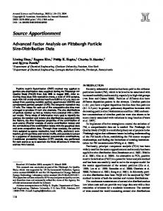
Fig. 1. Modeling domain with locations of the 8 receptors selected: Chicago PM2.5 nonattainment area (CNAA), St. Louis PM2.5 nonattainment area (SNAA), Mingo wilderness area (MING), Hercules-Glades wilderness area (HEGL), Upper Buffalo wilderness area (UPBU), Caney Creek wilderness area (CACR), Mammoth Cave national park (MACA), and Sipsey wilderness area (SIPS).

2. METHODS Both PSAT and DDM are implemented in CAMx and they can be compared using the same modeling framework. The details of the PSAT and DDM implementation in CAMx are given in the references mentioned above. Two month long (February and July) episodes from the St. Louis 36/12 km 2002 PM2.5 modeling database were selected for evaluating PSAT and DDM. Figure 1 shows the modeling domain. We selected 8 receptor locations that cover both urban (2 receptors) and rural (6 receptors) conditions for the analysis. In general, there was no notable distinction between the model results at the urban and rural sites with the only exception being PM2.5 ammonium which showed slightly more nonlinear responses to emission changes at the rural sites. Brute force emission reductions of 100% (zero-out) and 20% were simulated for the following anthropogenic emissions: SO2 and NOx from point sources; NOx, VOC, and NH3 from area sources (including mobile sources); all emission species from on-road mobile sources. BFM contributions were calculated by subtracting the PM concentrations of the emission reduction case from those of the base

concentration units and may be directly compared with the BFM response to 100% emissions reduction. Both quantities were linearly scaled for comparison with the 20% reduction BFM results. However, non-linear model response affects both the PSAT and DDM results, but in different ways. As illustrated in Figure 2, in a strongly non-linear system, the first-order DDM sensitivity is useful only for relatively small input changes while good agreement between PSAT and BFM is expected only near 100% emission reduction. The BFM inherently accounts for non-linear model response but may suffer limitations as a source apportionment method when the model response includes an indirect effect resulting from influence by chemicals other than the direct precursor. For example, consider an oxidant-limiting case of sulfate formation where oxidation of SO2 is limited by availability of H2O2 or O3. Removing an SO2 source in an oxidant-limited case makes more oxidant available to convert SO2 from other sources, resulting in a smaller zero-out contribution for the source than in an oxidant-abundant case. Furthermore, the sum of the zero-out contributions calculated separately for each source will likely not

2


add up to the total sulfate concentration in the base case. Indirect effects also can influence PSAT contributions for multi-pollutant sources where emissions of non-direct precursors have significant impact on the PM component of interest.

100% reduction

16

February

July

July 3 PSAT

PSAT

12

8

4

0 0

C3

4

8 BFM

12

16

0

100% reduction

16

C5 DDM

4

0 4

8 BFM

12

16

0

1

2 BFM

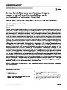
Fig. 3. Comparison of the PM2.5 sulfate changes (g/m3) due to reductions in point source SO2 emissions calculated by PSAT/DDM and BFM; each point represents the change in 24-hr average sulfate concentration due to the emission reduction at one receptor on one day. (A positive number means a decrease in ambient sulfate with the decrease in emissions).

Emissio

Fig. 2. Non-linear responses of pollutant concentration to emission reductions: ΔC1 and ΔC2 represent the changes in the pollutant concentration due to 100% reduction in the emission (from E0 to 0) estimated using zero-out BFM and first-order DDM sensitivity, respectively; if there exist no indirect effects, PSAT gives the same answer (ΔC1) as the BFM; ΔC3, ΔC4, and ΔC5 represent the model responses due to a smaller emission change (from E0 to E1) estimated by BFM, DDM, and PSAT, respectively.

100% reduction

1

February

July

July

PSAT

0.5

0.1

0

-0.5

3. RESULTS

-0.2 -1

-0.5

0 BFM

0.5

1

-0.2

100% reduction

1

Scatter plots comparing the PSAT (or DDM) and BFM results are shown in Figure 3 for the 8 receptor sites selected. With 100% reduction in the point source SO2 emissions, PSAT shows excellent agreement with the BFM in July while exhibiting slight over-estimation in February when oxidant-limiting effects are more important. With smaller (20%) reduction in point source SO2 emissions, the oxidant-limiting effect has greater impact because a greater fraction of the freed oxidant can oxidize SO2 from non-point sources (this happens because point sources dominate the SO2 emissions). This results in more difference between PSAT and BFM for 20% than 100% SO2 reduction. On the other hand, DDM and BFM agree better with 20% reduction than 100% as the model response becomes more linear with smaller input changes.

0

-0.1

-1

3.1 Sulfate

-0.1

0 BFM

0.1

0.2

20% reduction

0.2

February

February

July

July 0.1 DDM

0.5 DDM

20% reduction

0.2

February

PSAT

E0

4

2

1

0

E1

3

July

0

0

4

3

8

PSAT

3

20% reduction

July

C1

2 BFM

February

12

BFM

1

4

February

DDM

Pollutant Concentration

C2

C4

2

1

0

DDM

20% reduction

4

February

0

-0.5

0

-0.1

-1

-0.2 -1

-0.5

0 BFM

0.5

1

-0.2

-0.1

0 BFM

0.1

0.2

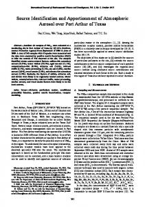
Fig. 4. Comparison of the PM2.5 sulfate changes (g/m3) due to reductions in on-road mobile source emissions calculated by PSAT/DDM and BFM; each point represents the change in 24-hr average sulfate concentration due to the emission reduction at one receptor on one day. (A positive number means a decrease in ambient sulfate with the decrease in emissions and a negative number an increase).

Scatter plots for sulfate changes due to reduced emissions of all species from mobile sources illustrate another indirect effect that is not accounted

3


by PSAT (Figure 4). Under winter condition (low temperature), more nitric acid can dissolve into water. Therefore, reducing mobile source NOx emissions decreases the acidity of the aqueous phase, which in turn increases sulfate concentrations as more SO2 dissolves and then is oxidized in the aqueous phase. In summer, reducing NOx emissions means less oxidant available to oxidize SO2, which decreases sulfate formation beyond reductions attributable to SO2 emissions reductions alone. However, because PSAT is designed to apportion PM to its primary precursor (in this case, sulfate is apportioned to SOx emissions and the indirect effect of reduced NOx emissions is ignored), the changes in sulfate estimated by PSAT are much smaller than those estimated using zero-out BFM in summer and even opposite direction in winter. The zero-out BFM is a sensitivity method and it is debatable whether the zero-out result can be considered a source apportionment in this case. DDM agrees much better with the zero-out result in this case because DDM can calculate sensitivity to multiple inputs and account for indirect effects.

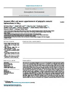
reduction of NH3 emissions from area sources, the changes in PM2.5 ammonium concentrations by PSAT are in excellent agreement with those by BFM while the DDM performance is impaired by nonlinearity in the gas-aerosol thermodynamic equilibrium for NH3 and ammonium. The same nonlinearity also weakens agreement between PSAT and BFM in the case of 20% emission reduction. Small emission changes can also emphasize any existing indirect effects (e.g., ammonium formation limited by sulfate or nitric acid). As seen in the above cases, the first-order DDM sensitivity performs well in describing model response to the smaller emission change. Comparison of PSAT and BFM for the changes in ammonium concentrations due to reduced mobile source emissions also shows the influence of indirect effects (not shown).

3.3 Nitrate Scatter plots shown in Figure 6 compare PM2.5 nitrate changes due to reductions in area NOx emissions. PSAT slightly over-estimates nitrate changes by zero-out BFM because availability of ammonia can limit nitrate partitioning into particle phase (similar to the effect of oxidant-limiting sulfate formation, discussed above).

3.2 Ammonium Figure 5 presents a clear example of the limitations of PSAT and DDM. With 100%

100% reduction

6 5

February 0.8

July

20% reduction

1

0.2

0

0 1

2

BFM

3

4

5

0.4 0.6 BFM

0.8

2 1

2

3 BFM

4

5

6

-0.2

100% reduction

4

1

July

0.4

0.2

0.4 BFM

0.6

0.8

1

0.8

1

20% reduction February

0.8

July

July

0.6

2 1

0.6

0

1

3

20% reduction

0.8

DDM

DDM

0.2

February

3

-0.2 1

February

1

July

0

5

February 4

0.2

1

0

0

100% reduction

5

0.4

2

0

0.4

1

3

DDM

2

0.6

DDM

3

0

July

0.8

PSAT

PSAT

February

July

4

PSAT

100% reduction February

July

0.6 PSAT

4 5

20% reduction

1

February

0.4 0.2

0

0

-1

-0.2 -1

0

1

2 BFM

3

4

5

-0.2

0

0.2

0.4 BFM

0.6

0.2

0

0 0

1

2

BFM

3

4

5

0

0.2

0.4 0.6 BFM

0.8

1

Fig. 5. Comparison of the PM2.5 ammonium changes 3 (g/m ) due to reductions in area source anthropogenic NH3 emissions calculated by PSAT/DDM and BFM; each point represents the change in 24-hr average ammonium concentration due to the emission reduction at one receptor on one day.

Fig. 6. Comparison of the PM2.5 nitrate changes (g/m3) due to reductions in area source anthropogenic NOx emissions calculated by PSAT/DDM and BFM; each point represents the change in 24-hr average nitrate concentration due to the emission reduction at one receptor on one day.

The differences between PSAT and BFM become larger for smaller emissions reduction due to the non-linear system. DDM again performs

4


better with smaller change in NOx emissions. Similar behaviors were observed with reductions in point source NOx emissions (not shown) although in this case the differences between PSAT and BFM for a 100% reduction in emissions are nearly as large as for a 20% reduction. Since NOx is the dominant component of on-road mobile source emissions, there is much less indirect effect due to other emission species from the sources. This explains relatively good agreement between PSAT and BFM in the case with all species from mobile emissions reduced (not shown).

4. DISCUSSION PSAT and DDM were applied in the same regional modeling framework to estimate the model responses to various BFM emission reductions by 100% and 20%. The results demonstrate that source sensitivity and source apportionment are equivalent for pollutants that are linearly related to emissions but otherwise differ because of non-linearity and/or indirect effects. Based on the simulations conducted in this study, the first-order DDM sensitivities can adequately predict the model responses of inorganic secondary aerosols to 20% emission changes (and, in some cases, larger changes). For SOA and primary aerosols, DDM agreed reasonably well with BFM up to 100% emission reductions. The DDM also gave reasonably good predictions for the impact of removing 100% of on-road mobile source emissions (all VOC, NOx, and particulate emissions) because the DDM accounts for indirect effects. However, as the size of model input changes increases, higher-order sensitivities become more important in general, and first-order sensitivity alone is not adequate to describe the model response for all magnitudes of emission reductions for all sources. Source apportionment by PSAT could successfully approximate the zero-out contributions for primary aerosols. Results for ammonium demonstrate that PSAT source apportionment and zero-out are nearly equivalent in a case (reduction in area source NH3 emissions) where the emissionsconcentration relationship is highly non-linear, but there is no indirect effect. Results for sulfate demonstrate that indirect effects (i.e., oxidant-limited sulfate formation) can limit the ability of zero-out to provide source apportionment and, therefore, that PSAT and zero-out may disagree when there are indirect effects. Neither PSAT nor first-order sensitivities provide an ideal method to relate PM components to sources. PSAT is best at apportioning sulfate, nitrate, and ammonium to sources emitting SO2, NOx, and NH3, respectively. PSAT is also better at estimating the impact on PM concentrations of removing all emissions from a source than removing a fraction of the emissions. First-order sensitivities are more accurate than PSAT in determining the impact of emissions that have indirect effects on secondary PM. This is especially true for sources such as motor vehicles that have substantial emissions of multiple pollutants (e.g., VOC and NOx) because complicated indirect effects are more likely for such sources. In contrast to PSAT, first-order sensitivities are better at estimating the effects of

3.4 Secondary Organic Aerosol (SOA) Both PSAT and DDM perform well in predicting the BFM responses of SOA concentrations to reductions in anthropogenic VOC emissions from area sources (not shown). DDM shows good performance even with 100% emission reduction demonstrating that the SOA module in CAMx responded nearly linearly to this emission change. PSAT also shows reasonable agreement with BFM for both 100% and 20% reductions probably because enough oxidant is available to convert VOC precursors to SOA and there are minimal indirect effects (although a hint of the oxidant-limiting effect can be seen in February). However, reducing NOx as part of mobile source emission reductions can significantly alter ambient oxidant levels, which changes SOA formation from not only anthropogenic but also biogenic VOC precursors. Source apportionment by PSAT excludes this kind of indirect effect, and thus significantly under-estimates the model response by BFM in summer when mobile source NOx emissions influence oxidants strongly (not shown).

3.5 Primary PM Since the source-receptor relationship for primary PM is essentially linear and not affected by any indirect effects, it is expected that both PSAT and DDM should accurately predict the model response of primary PM species to their emissions. Excellent agreement was found between PSAT (or DDM) and BFM for changes in primary PM2.5 concentrations from mobile sources (not shown).

5


air quality model. Environ. Sci. Technol. 36, 2953-2964. Hakami, A., M.T. Odman and A.G. Russell. 2003. High-order, direct sensitivity analysis of multidimensional air quality models. Environ. Sci. Technol. 37, 2442-2452. Kleeman, M.J., G.R. Cass and A. Eldering. 1997. Modeling the airborne particle complex as a source-oriented external mixture. J. Geophys. Res. 102, 21355-21372. Koo, B., A.M. Dunker and G. Yarwood. 2007. Implementing the Decoupled Direct Method for sensitivity analysis in a particulate matter air quality model. Environ. Sci. Technol. 41, 2847-2854. Koo, B., G. Yarwood and D.S. Cohan. 2008. HigherOrder Decoupled Direct Method (HDDM) for ozone modeling sensitivity analyses and code refinements. Final Report prepared for Texas Commission on Environmental Quality, Austin, TX. Koo, B., G.M. Wilson, R.E. Morris, G. Yarwood and A.M. Dunker. 2009. CRC Report No. A-64: Evaluation of CAMx probing tools for particulate matter. Final Report prepared for Coordinating Research Council, Alpharetta, GA (www.crcao.com). Napelenok, S.L., D.S. Cohan, Y. Hu, and A.G. Russell. 2006. Decoupled direct 3D sensitivity analysis for particulate matter (DDM-3D/PM). Atmos. Environ. 40, 6112-6121. Tonnesen, G. and B. Wang. 2004. CMAQ Tagged Species Source Apportionment (TSSA). Presented at the WRAP Attribution of Haze Workgroup Meeting, Denver, CO. www.wrapair.org/forums/aoh/meetings/04072 2/UCR_tssa_tracer_v2.pdf Wagstrom, K.M.; S.N. Pandis, G. Yarwood, G.M. Wilson and R.E. Morris. 2008. Development and application of a computationally efficient particulate matter apportionment algorithm in a three-dimensional chemical transport model. Atmos. Environ. 42, 5650-5659. Yang, Y.. J.G. Wilkinson and A.G. Russell. 1997. Fast, direct sensitivity analysis of multidimensional photochemical models. Environ. Sci. Technol. 31, 2859-2868.

eliminating a fraction of emissions from a source than eliminating all emissions from the source. Both PSAT and first-order sensitivities are accurate for apportioning primary PM to emission sources. To some extent, PSAT and first-order sensitivities are complementary methods. Depending on which PM components, sources and magnitude of emission reductions are being examined, the considerations given above can be used as a guide in deciding which method to apply, PSAT or first-order sensitivities. Although we have used the BFM as a standard against which to compare the two other methods, it too has limitations. It is the most computationally expensive when determining the contributions of multiple sources. Also, the BFM is normally applied by removing each source individually from the base case, e.g., base case minus source i to determine the contribution of source i. Whenever model response is nonlinear, e.g., due to chemistry, the sum of these source contributions will not add up to the simulated concentrations in the base case.

5. ACKNOWLEDGMENTS This work was funded by the Coordinating Research Council under Project A-64.

6. REFERENCES Cohan, D.S., A. Hakami, Y. Hu and A.G. Russell. 2005. Nonlinear response of ozone to emissions: source apportionment and sensitivity analysis. Environ. Sci. Technol. 39, 6739-6748. Dunker, A. M. 1980. The response of an atmospheric reaction-transport model to changes in input functions. Atmos. Environ. 14, 671-679. Dunker, A. M. 1981. Efficient calculation of sensitivity coefficients for complex atmospheric models. Atmos. Environ. 15, 1155-1161. Dunker, A.M., G. Yarwood, J.P. Ortmann and G.M. Wilson. 2002a. The Decoupled Direct Method for sensitivity analysis in a three-dimensional air quality model – implementation, accuracy, and efficiency. Environ. Sci. Technol. 36, 2965-2976. Dunker, A.M., G. Yarwood, J.P. Ortmann and G.M. Wilson. 2002b. Comparison of source apportionment and source sensitivity of ozone in a three-dimensional

6