Int. J. Contemp. Math. Sciences, Vol. 6, 2011, no. 9, 409 - 421
Comparison of Robust Regression Methods in Linear Regression Özlem Gürünlü Alma Muğla University, Faculty of Arts & Sciences Department of Statistics, Muğla, Turkey
[email protected] Abstract In classical multiple regression, the ordinary least squares estimation is the best method if assumptions are met to obtain regression weights when analyzing data. However, if the data does not satisfy some of these assumptions, then sample estimates and results can be misleading. Especially, outliers violate the assumption of normally distributed residuals in the least squares regression. The danger of outlying observations, both in the direction of the dependent and explanatory variables, to the least squares regression is that they can have a strong adverse effect on the estimate and they may remain unnoticed. Therefore, statistical techniques that are able to cope with or to detect outlying observations have been developed. Robust regression is an important method for analyzing data that are contaminated with outliers. It can be used to detect outliers and to provide resistant results in the presence of outliers. The purpose of this study is to define behavior of outliers in linear regression and to compare some of robust regression methods via simulation study. The simulation study is used in determining which methods best in all of the linear regression scenarios. Keywords: Least Trimmed Squares M, Yohai MM estimate, S estimate, Robust Regression, Outlier, Ordinary Least Square
1 Introduction Regression is one of the most commonly used statistical techniques. Out of many possible regression techniques, the ordinary least squares (OLS) method has been generally adopted because of tradition and ease of computation. However, OLS estimation of regression weights in the multiple regression are affected by the occurrence of outliers, non-normality, multicollinearity, and missing data [9].
410
Ö. Gürünlü Alma
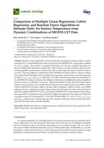
As defined by Barnett and Lewis (1994), outliers are observations that appear inconsistent with the rest of the data. Often, such influential points remain hidden to the user, because they do not always show up in the usual least squares residual plots. To remedy this problem, new statistical techniques have been developed that are not so easily affected by outliers. These are robust methods, such as Least Median of Squares (LMS), Least Trimmed Squares (LTS), Huber M Estimation, MM Estimation, Least Absolute Value Method (LAV) and S Estimation [3, 4, 18, 20]. The main purpose of robust regression is to provide resistant results in the presence of outliers. In order to achieve this stability, robust regression limits the influence of outliers. Figure 1 illustrates the different types of outliers. The ellipse defines the majority of the data. Points A, B, and C are outliers in Yspace because their y values or response values are significantly different from the rest of the data and they are also residual outliers. Points B, C and D are outliers in X-space, that is, their x values are unusual and these are also referred to as leverage points. Although D is outlying in X-space, it is not a residual outlier. Points B and C are leverage points and residual outliers. Point A is an inlier in X-space but a residual outlier. Point E is an inlier in Y-space and also a residual outlier [1].
Figure 1. Scatter plot for the different type of outlying observations
All these different types of outliers can be summarized as in Table 1 [1]. Table 1. Different Types of Outliers Points Y-space outlier X-space outlier A * B * * C * * D * * E *
Residual outlier * * * *
The purpose of this study was to compare robust regression methods; LTS, M estimate, Yohai MM estimate, and S estimate against OLS regression estimation method in terms of the determination of coefficient. For this
Comparison of robust regression methods
411
purpose, it was reviewed the leverage points, breakdown point, and the relative efficiency of a robust regression estimator in Section 2. After giving a brief description of outliers in regression analysis, in the following section, detailed explanation of the robust regression methods will be presented in Section 3. The data simulation procedure used to study the performances of these methods was described in Section 4 and, also comparison results of simulation study are described in this section.
2 Outliers in Multiple Linear Regression The multiple linear regression model in terms of the observations can be written as matrices notation by y = Xβ + ε , where y is an n × 1 vector of observed response values, X is the n × p matrix of the predictor variables, β is the p × 1 , and ε is the n × 1 vector of random error terms. The aim of regression analysis is to find the estimates of unknown parameters. The OLS is used to find the best estimate of β ’s with the least squares criterion which minimizes the sum of squared distances of all of the points from the actual observation to the regression surface [7]. It often happens in practice that an assumed normal distribution model (e.g., a location model or a linear regression model with normal errors) holds approximately in that it describes the majority of observations, but some observations follow a different pattern or no pattern at all. In the case when the randomness in the model is assigned to observational errors which was the first instance of the use of the least-squares method, the reality is that while the behavior of many sets of data appeared rather normal, this held only approximately, with the main discrepancy being that a small proportion of observations were quite atypical by virtue of being far from the bulk of the data. Behavior of this type is common across the entire spectrum of data analysis and statistical modeling applications. Such atypical data or even a single outlier can have a large distorting influence on a classical statistical method that is optimal under the assumption of normality or linearity. The primary purpose of robust regression techniques is to fit a model that describes the information in the majority of the data. This general definition implies that these techniques should perform well on both with outliers and on without outliers [8].
3 Robust Regression Methods Robust regression analysis provides an alternative to a least squares regression when fundamental assumptions are unfulfilled by the nature of the data [11]. The properties of efficiency, breakdown, and high leverage points are used to define robust techniques performance in a theoretical sense. One aim of robust estimators is a high finite sample breakdown point ε *n defined by
412
Ö. Gürünlü Alma
Donoho & Huber, in 1983 [6]. The breakdown point can be defined as the point or limiting percentage of contamination in the data at which any test statistics first becomes swamped. Hence, the breakdown point is simply the initial point at which any statistical test becomes swamped due to contaminated data. Some regression estimators have the smallest possible breakdown point of 1/n or 0/n. In other words, only one outlier would cause the regression equation to be rendered useless. Other estimators have the highest possible breakdown point of n/2 or 50%. If robust estimation technique has a 50% breakdown point then 50% of the data could contain outliers and the coefficients would remain useable [5, 14] state: Take any sample of n data points, (1)
Z={(x11,…,x1p,y1),…,(xn1,…,xnp,yn)}
and let T be a regression estimator. This means that applying T to such a sample Z yields a vector of regression coefficients. Now consider Z that are obtained by replacing any of m the original data points by arbitrary values. Let us denote by bias (m;T,Z) the maximum bias (2)
bias(m; T.Z) = sup || T(Z′) − T(Z) ||
where the supremum is over all possible Z. If bias (m;T,Z) is infinite, this means that m outliers can have an arbitrary large effect of T which may be expressed by saving that estimator breaks down. Therefore, the (finite-sample) breakdown point of the estimator T at the sample Z is described as follows, ε′(T, Z) = min{m / n; bias(m; R, Z)}
is
infinite .
(3)
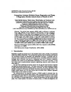
In other words, it is the smallest fraction of contamination that can cause the estimator T to take on values arbitrarily far from T(Z). For least squares, we have seen that one outlier is sufficient to carry T over all bounds. Therefore, its breakdown point is ε′(T, Z) = 1/ n . The leverage point is an observation (xp,yp) which a whenever xp lies far away from the bulk of the observed xi in the sample [16], it is seen in Figure 2.
Figure 2.The point (xp,yp) is leverage point because xp is outlying. However, (xp,yp) is not a regression outlier because it matches the linear pattern set by the other data points.
Comparison of robust regression methods
413
In general, most robust regression models can be divided into three broad categories; M, L, and R estimation models. Each category contains a class of models derived under similar conditions and with comparable theoretical statistical properties. Least Trimmed Squares Estimate, M-Estimate, Yohai MM-Estimate and S-Estimate are used in this study and, they are briefly described in the following subsections.
3.1 Least Trimmed Squares (LTS) Estimate Rousseeuw (1984) developed the least trimmed squares (LTS) estimation method and this method is given by, h
βˆ LTS = arg min Q LTS (β) where Q LTS (β) = ∑ ei2
(4)
i =1
e (21) ≤ e (22 ) ≤ ... ≤ e (2n ) are the ordered squared residuals, from smallest to largest.
LTS is calculated by minimizing the h ordered squares residuals, where h= [n/2]+[(p+1)/2], with n and p being sample size and number of parameters, respectively. The largest squared residuals are excluded from the summation in this method, which allows those outlier data points to be excluded completely. Depending on the value of h and the outlier data configuration, LTS can be very efficient. In fact, if the exact numbers of outlying data points are trimmed, this method is computationally equivalent to OLS. However, if there are more outlying data points than are trimmed, this method is not as efficient. Conversely, if there is more trimming than there are outlying data points, then some good data will be excluded from the computation. In terms of breakdown, LTS is considered to be a high breakdown method with a breakdown point of 50% [14, 15].
3.2 M Estimate The class of M-estimator models contains all models that are derived to be maximum likelihood models. The most common general method of robust regression is M-estimation, introduced by Huber (1964) that is nearly as efficient as OLS [10]. Rather than minimize the sum of squared errors as the objective, the M-estimate minimizes a function ρ of the errors. The M-estimate objective function is, n n e y − x ′i βˆ min ∑ ρ( i ) = min ∑ ρ( i ) s s i =1 i =1
(5)
where s is an estimate of scale often formed from linear combination of the residuals. The function ρ gives the contribution of each residual to the objective function. A reasonable ρ should have the following properties: ρ(e)≥0 ,ρ(0)=0 ,ρ(e)= ρ(-e), and ρ(ei) ≥ ρ(e′i) for |ei| ≥ |e′i|. For example, for least squares estimation, ρ(ei) = ei2. The system of normal equations to solve this minimization problem is found by taking partial derivatives with respect to β and setting them equal to 0, yielding,
414
n
∑ ψ( i =1
Ö. Gürünlü Alma
yi − x ′βˆ i )x i = 0 s
(6)
where ψ is derivative of ρ. The choice of the ψ function is based on the preference of how much weight to assign outliers. A monotone ψ function does not weight large outliers as much as least squares (e.g. 10σ outlier would receive the same weight as a 3σ outlier). A redescending ψ function increases the weight assign to an outlier until a specified distance (e.g.3σ) and then decreases the weight to 0 as the outlying distance gets larger. Newton-Raphson and Iteratively Reweighted Least Squares (IRLS) are the two methods to solve the Mestimates nonlinear normal equations. IRLS expresses the normal equations as, X′WXβˆ = X ′Wy
(7)
where W is an n x n diagonal matrix of weights, ⎡ Y − x ′i βˆ 0 ⎤ ⎡ Yi − x ′i βˆ 0 ⎤ wi = ψ ⎢ i ⎥/⎢ ⎥ s s ⎢⎣ ⎥⎦ ⎢⎣ ⎥⎦ .
(8)
The initial vector of parameter estimates, βˆ 0 , are typically obtained from OLS. IRLS updates these parameter estimates with βˆ 1 = ( X ′WX) −1 ) X′Wy .
(9)
The weights, however, depend upon the residuals, the residuals depend upon the estimated coefficients, and the estimated coefficients depend upon the weights. An iterative solution called iteratively re-weighted least squares, IRLS is therefore required: 1. Select initial estimates b(0), such as the least squares estimates, 2. At the each iteration t, calculate residuals ei(t-1) and associated weights ωi(t −1) = ω[ei(t −1) ] from the previous iteration, 3. Solve for new weighted least squares estimates ( t −1) (t ) (t −1) −1 ( t −1) (t −1) b = [X′W X] X ′W Y , and W =diag{ ωi } is the current weight matrix. Step2 and Step3 are repeated until the estimated coefficient converge. The procedure continues until some convergence criterion is satisfied. The estimate of scale may be updated after initial estimate. However M-estimators are not robust to x-axis outlier data values, their breakdown point is 1/n.
415
Comparison of robust regression methods
3.3 Yohai MM Estimate MM estimation is a special type of M-estimation developed by Yohai (1987) [22]. MM-estimation is a combination of high breakdown value estimation and efficient estimation Yohai's MM estimator was the first estimate with a high breakdown point and high efficiency under normal error [19]. MM-estimators have three stage procedures. 1. The first stage is calculating an S-estimate with influence function 2
4
⎛x⎞ ⎛x⎞ ⎛x⎞ ρ(x) = 3 ⎜ ⎟ − 3 ⎜ ⎟ + ⎜ ⎟ c ⎝ ⎠ ⎝c⎠ ⎝c⎠
6
if x ≤ c, otherwise ρ(x) = 1.
(10)
The value of tuning constant, c, is selected as 1.548. 2. The second stage calculates the MM parameters that provide the n ⎛ y − x ′i βˆ MM ⎞ ⎟ where ρ(x) is the influence minimum value of ∑ ρ⎜⎜ i ⎟ σˆ 0 i =1 ⎝ ⎠
function used in the first stage with tuning constant 4.687 and σˆ 0 is the estimate of scale form the first step (standard deviation of the residuals). 3. The final step computes the MM estimate of scale as the solution to (11)
1 n ⎛ y i − x ′i βˆ ⎞ ∑ ρ ⎜ s ⎟⎟ = 0.5 n − p i =1 ⎜⎝ ⎠
3.4 S-Estimate S estimation is a high breakdown value method introduced by Rousseeuw and Yohai (1984) that minimizes the dispersion of the residuals [13]. The objective function is min s(e1 (β),..., e n (β)) where ei (β) is the ith residuals for candidate β. This objective function is given by the solution, ˆ 1 n ⎛ Yi − Y i χ ⎜⎜ ∑ n − p i =1 ⎝ s
⎞ ⎟⎟ = K ⎠
(12)
where K is a constant E φ [ρ] with φ defined as the standard normal. Rousseeuw and Yohai (1984) suggest a redescending influence function as, ρ(x) = {
x2 x4 x6 − 2+ 4 2 2c 6c
if x ≤ c,
otherwise ρ(x) =
c2 . 6
(13)
The parameter c is the tuning constant. Tradeoffs in breakdown and efficiency are possible based on choices for tuning constant c and K. The usual choice is c=1,548 and K=0,1995 for 50% breakdown and about 28% asymptotic efficiency [14]. The final scale estimate, s, is the standard deviation of the residuals from the fit that minimized the dispersion of the residuals.
416
Ö. Gürünlü Alma
4 Data Simulation and Comparisons of the Methods In this study, four robust regression methods were comparatively evaluated against OLS regression method. These robust methods are the most commonly used regression method when data contains outliers. OLS is compared to highly regard robust methods in terms of efficiency, breakdown, leverage points and coefficient of determination. One of the effective performance statistics is the coefficient of determination (R-square). R-square is the statistic that will give information about the goodness of fit of the model that is found by R 2 =
SSRe gression SSTotal
= 1−
SSError . This coefficient is used to comparison of OLS with SSTotal
robust regression estimates in linear regression models. The data sets are generated from the model yi = β0 +β1 x i1 +...+ ei , i=1,...,n where all regression coefficients are fixed β j = 5, for each i=1,...,n and j=1,...,p and the errors are assumed to be independent. The explanatory variables x ij ∈ ℜ n × p are sampled independently from a N(0,1). The sample data sets are generated under the sample sizes are fixed, n = 30. To change the place of good data points a specified number of standard deviations away from the lie of the best fit created x-axis or y-axis outlier data. Outliers were placed in two different locations to simulate different types of outliers. These placements of data points represent both x-axis and y-axis outliers (2x, 2y, σ; 4x, 4y, σ) . The program code for the data simulation and outlier generation was adapted in SAS [17, 21]. And also, for the study included following conditions; number of explanatory variables, outlier density and outlier location. The regression equations included 2, 3, and 5 explanatory variables. Outlier density was zero, five, and ten. Outlier location included two levels. Each of the data configurations was used to compare OLS with the four robust regression estimates techniques. The variation in comparison of robust regression methods provides an indication of the sensitivity of the methods. The simulation results, R2 values of robust methods are obtained from 1.000 replications, and performances comparisons of methods are as following;
4.1 Efficiency Datasets used for the efficiency test are only x1 has leverage points, only x2 has leverage points, both x1-x2 have leverage points and y have no outlier points. One thousands replications of each treatment combination are run to obtain R-square values for each technique in SAS. A means of evaluating robust method efficiencies is to compares their performances relative to least squares using simulation data. The regression model was selected as yi = 5 + 5x1i + 5x 2i +0.5εi . Errors and explanatory variables generated from random normal varieties. Data was simulated from a normal distribution with a mean of zero and a standard deviation of one. Number of leverage points is varied so that changes in estimation behavior can be evaluated. R2
417
Comparison of robust regression methods
values of robust methods are evaluated, including known high and low efficiency techniques. Table 2 lists the R-square results for each design. Table 2. Robust Techniques Performances against OLS
R2 values
Properties of Dataset 5% leverage points and No outlier
Variables x1 x2 x1 – x2 -y
OLS 0.0016 0.0086 0.0050
LTS 0.1924 0.2192 0.2333
M 0.0016 0.0085 0.0050
MM 0.0562 0.0082 0.0050
S 0.9921 0.9914 0.9921
10% leverage points and No outlier
x1 x2 x1 – x2 -y Sum
0.0015 0.0015 0.0001 0.0183
0.1961 0.1996 0.1755 1.2161
0.0015 0.0015 0.0020 0.0201
0.0015 0.0015 0.0025 0.0749
0.2019 0.7348 0.0177 3.93
From Table 2, M and MM estimators perform the most like least squares regardless of the presence of leverage points in axis. The fits for M- and MMestimation fail because their objective functions do not bound the influence of the high leverage points. LTS has low determination of coefficient, and then it is not good estimation of parameters. S estimator method performs better than other methods when the data has high leverage points. For the high percentage of X’s leverage points S estimator method performs like LTS method.
4.2 Breakdown The breakdown of various robust methods is typically measured for a certain sample size. To fully challenge the robust methods, designs are developed with a percentage of outliers and percentage of leverage points. The six-variable problem has 5% leverage points and either 10% or 15% outliers in y axis, for 2,3,5 explanatory variables with intercept in model. Table 3 lists the R-square results for each design. Table 3. Robust Techniques Performances against OLS Properties of Dataset 5% leverage points and 10% outliers 5% leverage points and 15% outliers
# of Explanatory Variables 2 3 5 2 3 5 Sum
R2 values
OLS
LTS
M
MM
S
0.0865 0.1380 0.2598
0.9955 0.9969 0.9982
0.8288 0.8392 0.8385
0.3411 0.4385 0.3332
0.9953 0.9969 0.9982
0.0341 0.0783 0.1322 0.7289
0.9954 0.9970 0.9982 5.9812
0.7893 0.7974 0.7974 4.8906
0.0952 0.1392 0.1341 1.4813
0.9952 0.9969 0.9983 5.9808
The Table 3 is shown MM-estimators perform the most like least squares regardless of the presence of leverage points and outliers in y axis. LTS has high determination of coefficient, and then it is good estimation of parameters. S estimator is better than M estimator. MM estimator is also known high breakdown value estimation but it is not efficiency estimator this design. From
418
Ö. Gürünlü Alma
Table 3, the best estimator methods are LTS and S method, these methods perform better than other methods. The main purpose of robust regression is to provide resistant results in the presence of outliers so these methods is also compared difference percentage of outliers in y variable which have 10%, 25%, and 40% outliers each of design. The results of these simulations are given in Table 4.
Table 4. Robust Techniques Performances
Percentage of outliers in y variables 10 25 40 Sum
OLS
LTS
0.0342 0.0183 0.0059 0.0584
0.09956 0.08784 0.2598 0.4472
R2 values M 0.7894 0.6639 0.0055 1.4588
MM 0.7605 0.0489 0.0056 0.8150
S 0.9952 0.2927 0.0078 1.2957
Generally the least efficient method was the OLS and LTS method for this design. Huber M estimation is good estimator other than methods especially data has outliers and no leverage points. S estimation is a high breakdown value method, which has a higher statistically efficient than MM and LTS. For the low percentage of outliers in y variables S estimator method performs much better than other methods, but all methods perform are decreasing when the percentage of outliers are increasing.
5 Conclusion In this study, four robust regression methods were comparatively evaluated against OLS regression method. S estimator has reasonable efficiencies, bound the influence of high leverage outliers, and demonstrate high breakdown. Huber M estimator is efficient outliers. For 10% breakdown S-estimator would increase its efficiency. MM-estimation performs the best overall against a comprehensive set of outlier conditions. However, MM-estimation has trouble with high leverage outliers in small to moderate dimension data. These simulation data are a good illustration of MM-estimation’s weakness. Table 5 shows comparisons of all results, as seen from this table S and M estimator methods perform better than LTS and MM estimator methods.
Comparison of robust regression methods
419
References [1] R. Adnan, M.N. Mohamad, and H. Setan, Multiple outliers detection procedures in linear regression. Matematika, Jabatan Matematik, UTM., 19(1) (2003), 29-45. [2] V. Barnett and T. Lewis, Outliers in Statistical Data, John Wiley and Sons, USA, 1998. [3] R.A. Berk, A Primer on Robust Regression. In J. Fox and J.S. Long (Editors), Modern Methods of Data Analysis Newbury Park, CA: Sage Publications, Inc, (pp. 292-323), 1990. [4] D. Birkes and Y. Dodge, Alternative Methods of Regression, John Wiley&Sons, Canada, 1993. [5] A. Christmann, Least median of weighted squares in logistic regression with large strata. Biometrika 81 (1994), 413-417. [6] D.L. Donoho and P.J. Huber, The notion of breakdown point. In: Bickel PJ, Doksum KA, Hodges JL Jr (Editors), A Festschrift for Erich L. LehmannWadsworth, Belmont,( pp 157-184), 1983. [7] J. Fox, Applied Regression Analysis, Linear Models and Related Methods, 3th ed., Sage Publication, USA, 1997. [8] F.R Hampel, E.M. Ronchetti, P.J. Rousseeuw, and W.A. Stahel, Robust Statistics. The Approach Based on Influence Functions, John Wiley and Sons, New York, 1986. [9] K. Ho, J. Naugher, Outliers lie: An illustrative example of identifying outliers and applying robust models. multiple linear regression viewpoints, 26(2) (2000), 2-6. [10] P.H. Huber, Robust estimation of a location parameter, The Annals of Mathematical Statistics, 35 (1964), 7-101.
420
Ö. Gürünlü Alma
[11] R. Marona, R. Martin, V.J. Yohai, Robust Statistics Theory and Methods, John Wiley & Sons Ltd., England, 2006. [12] P.J. Rousseeuw, Least median of squares regression, Journal of the American Statistical Association, 79 (1984), 871-880. [13] P.J. Rousseeuw, and V. Yohai, Robust regression by means of Sestimators. In W. H. J. Franke and D. Martin (Editors.), Robust and Nonlinear Time Series Analysis, Springer-Verlag, New-York, (pp. 256272), 1984. [14] P.J. Rousseeuw, A.M. Leroy, Robust Regression and Outlier Detection. Wiley-Interscience, New York, 1987. [15] P.J.Rousseeuw, K. Van Driessen, Computing LTS regression for large data sets, Technical Report, University of Antwerp, 1998. [16] P.J. Rousseeuw, A Diagnostic plot for regression outliers and leverage points, Computational Statistics and Data Analysis, 11 (1991), 127-129. [17] SAS Institute Inc., Robust Regression and Outlier Detection with the Robustreg Procedure, USA, 2006. [18] R.G. Staudte and S.J Sheatherm, Robust Estimation and Testing, John Wiley &Sons, New York, 1990. [19] A.J. Stromberg, Computation of high breakdown nonliner regression parameters, Journal of the American Statistical Association, 88(421), (1993). [20] R.R. Wilcox, Introduction to Robust Estimation and Hypothesis Testing, CA:Academic Press, San Diego, 1997. [21] R. Yaffee, Robust Regression Analysis: Some Popular Statistical Package Options, (2002). Available at: http://www.nyu.edu/its/statistics/Docs/RobustReg2.pdf (17 September 2010) [22] V.J. Yohai, High breakdown-point and high effciency robust estimates for regression, The Annals of Statistics, 15 (1987), 642-656.
Appendix: SAS codes data a (drop=i); do i=1 to 1000; x1=rannor(1234); x2=rannor(1234); e=rannor(1234); if i > 900 then y=100 + e; else y=5 + 5*x1 + 5*x2 + .5 * e; output; end; run; proc reg data=a; model y = x1 x2 ;run; proc robustreg data=a; model y = x1 x2 / diagnostics leverage; output out=robout r=resid sr=stdres; run; proc robustreg data=a; method=lts ; model y = x1 x2 ; run; proc robustreg data=a; method=m (wf=huber(c=2)); model y = x1 x2 ; run; proc robustreg data=a; method=mm (chif=yohai inith=502 k0=1.8); model y = x1 x2; run; proc robustreg data=a; method=s; model y = x1 x2; run; ods html; ods graphics on; proc robustreg data=a; plots=(rdplot ddplot reshistogram resqqplot); model y = x1 x2; run;
Comparison of robust regression methods
421
ods graphics off; ods html close; data a (drop=i); do i=1 to 1000; x1=rannor(1234); x2=rannor(1234); x3=rannor(1234); e=rannor(1234); if i > 900 then y=100 + e; else y=5 + 5*x1 + 5*x2 + 5*x3 + .5 * e; output; end; run; proc reg data=a; model y = x1 x2 x3 ; run; proc robustreg data=a; model y = x1 x2 x3 / diagnostics leverage; output out=robout r=resid sr=stdres; run; proc robustreg data=a; method=lts ; model y = x1 x2 x3 ; run; proc robustreg data=a; method=m (wf=huber(c=2)); model y = x1 x2 x3 ; run; proc robustreg data=a; method=mm (chif=yohai inith=502 k0=1.8); model y = x1 x2 x3;run; proc robustreg data=a; method=s; model y = x1 x2 x3; run; ods html; ods graphics on; proc robustreg data=a; plots=(rdplot ddplot reshistogram resqqplot); model y = x1 x2 x3;run; ods graphics off; ods html close; data a (drop=i); do i=1 to 1000; x1=rannor(1234); x2=rannor(1234); x3=rannor(1234); x4=rannor(1234); . x5=rannor(1234); e=rannor(1234); if i > 900 then y=100 + e; else y=5 + 5*x1 + 5*x2 + 5*x3 + 5*x4 + 5*x5 +.5 * e; output; end; run; proc reg data=a; model y = x1 x2 x3 x4 x5;run; proc robustreg data=a; model y = x1 x2 x3 x4 x5 / diagnostics leverage; output out=robout r=resid sr=stdres; run; proc robustreg data=a; method=lts ; model y = x1 x2 x3 x4 x5; run; proc robustreg data=a; method=m (wf=huber(c=2));model y = x1 x2 x3 x4 x5; run; proc robustreg data=a; method=mm (chif=yohai inith=502 k0=1.8); model y = x1 x2 x3; run; proc robustreg data=a; method=s; model y = x1 x2 x3 x4 x5; run; ods html; ods graphics on; proc robustreg data=a; plots=(rdplot ddplot reshistogram resqqplot); model y = x1 x2 x3 x4 x5; run; ods graphics off; ods html close;
Received: September, 2010