Computers and Chemical Engineering 24 (2000) 175 – 181 www.elsevier.com/locate/compchemeng
Comparison of statistical process monitoring methods: application to the Eastman challenge problem Manabu Kano a,*, Koji Nagao a, Shinji Hasebe a, Iori Hashimoto a, Hiromu Ohno b, Ramon Strauss c, Bhavik Bakshi c a Department of Chemical Engineering, Kyoto Uni6ersity, Kyoto, Japan Department of Chemical Science and Engineering, Kobe Uni6ersity, Kobe, Japan c Department of Chemical Engineering, The Ohio State Uni6ersity, Ohio, OH, USA b
Abstract Multivariate statistical process control (MSPC) has been successfully applied to chemical processes. In order to improve the performance of fault detection, two kinds of advanced methods, known as moving principal component analysis (MPCA) and DISSIM, have been proposed. In MPCA and DISSIM, an abnormal operation can be detected by monitoring the directions of principal components (PCs) and the degree of dissimilarity between data sets, respectively. Another important extension of MSPC was made by using multiscale PCA (MS-PCA). In the present work, the characteristics of several monitoring methods are investigated. The monitoring performances are compared with using simulated data obtained from the Tennessee Eastman process. The results show that the advanced methods can outperform the conventional method. Furthermore, the advantage of MPCA and DISSIM over conventional MSPC (cMSPC) and that of the multiscale method are combined, and the new methods known as MS-MPCA and MS-DISSIM are proposed. © 2000 Elsevier Science Ltd. All rights reserved. Keywords: Fault detection; Monitoring; Statistical process control; Pattern recognition; Principal component analysis; Wavelet analysis
1. Introduction For a successful operation of any process, it is important to detect process upsets, equipment malfunctions, or other special events as early as possible and then to find and remove the factors causing those events. In chemical processes, databased approaches rather than model-based approaches have been widely used for process monitoring, because it is often difficult to develop detailed physical models. The data-based approaches are referred to as statistical process control (SPC), and conventional SPC charts such as Shewhart chart and CUSUM chart have been widely used. Such SPC charts are well established for monitoring univariate processes, but they do not function well for multivariable processes with highly correlated variables. In addition, chemical processes are becoming more heavily * Corresponding author. Present address: Department of Chemical Engineering, Ohio State University, 140 W 19th Avenue, Columbus, OH 43210, USA.. E-mail address:
[email protected] (M. Kano).
instrumented, and the data are more frequently recorded. This causes a data overload, and a great deal of data is wasted. Therefore, in order to extract useful information from process data and utilize it for process monitoring, multivariate statistical process control (MSPC) has been developed (Kresta, MacGregor & Marlin, 1991). MSPC is based on the chemometric techniques such as principal component analysis (PCA) and partial least squares (PLS). Wise and Gallagher (1996) reviewed some of the chemometric techniques and their application to chemical process monitoring and dynamic process modeling. They defined chemometrics as the science relating measurements made on a chemical system to the state of the system via application of mathematical or statistical methods. Using multiway PCA and PLS (Wold, Geladi, Esbesen & Ohman, 1987), Nomikos and MacGregor (1994) extended the MSPC functioning to monitor time-varying batch processes. Another extension to handle very large processes via multiblock PCA and PLS was made by MacGregor, Jaeckle, Kiparissides and Koutoudi (1994). PCA has
0098-1354/00/$ - see front matter © 2000 Elsevier Science Ltd. All rights reserved. PII: S 0 0 9 8 - 1 3 5 4 ( 0 0 ) 0 0 5 0 9 - 3
176
M. Kano et al. / Computers and Chemical Engineering 24 (2000) 175–181
also been used for fault identification (Dunia, Qin, Edgar & McAvoy, 1996). PCA is a tool for data compression and information extraction. PCA finds linear combinations of variables that describe major trends in a data set. For monitoring a process with PCA, control limits are set for two kinds of statistic, T 2 and Q, after a PCA model is developed. A measure of the variation within the PCA model is given by Hotelling’s T 2 statistic. T 2 is the sum of normalized squared scores. On the other hand, Q is the sum of squared errors, and it is a measure of the amount of variation not captured by the PCA model. Many successful applications have shown the practicability of MSPC. The conventional MSPC (cMSPC) method described above, however, does not always function well, because it cannot detect any changes in the operating condition if the indexes are inside the control limits. In order to improve the performance of process monitoring, two kinds of statistical process monitoring methods were proposed by Kano, Nagao, Ohno, Hasebe & Hashimoto (1999, 2181). The first method was termed moving principal component analysis (MPCA). This method is based on the idea that changes in the operating condition, i.e. changes in the correlation among process variables, can be detected by monitoring directions of principal components (PCs). A new index was defined for evaluating the changes in the direction of each PC and the changes in the subspace spanned by selected PCs. The second method was termed DISSIM. This method is based on the idea that changes in the operating condition can be detected by monitoring a distribution of time-series data, which reflects the corresponding operating condition. In order to evaluate quantitatively the difference between two data sets, the dissimilarity index was defined. Another important extension of MSPC was made utilizing wavelet analysis. PCA has the ability to extract the relationship between variables and decorrelate the cross-correlation, and wavelet analysis has the ability to extract features in the measurements and approximately decorrelate the autocorrelation. Combining the above two functions, Bakshi (1998) developed multiscale PCA (MS-PCA). The MS-PCA method was applied to monitoring problems, and the superiority of process monitoring by MS-PCA over conventional PCA was illustrated. In the present work, the characteristics of several monitoring methods, including MPCA, DISSIM, and MS-PCA, are investigated. The performance of the monitoring methods are compared with using simulated data obtained from the Tennessee Eastman process. Furthermore, the advantage of MPCA or DISSIM over cMSPC and that of the multiscale method are combined, and the new methods named MS-MPCA and MS-DISSIM are proposed.
2. Advanced MSPC methods In this section, several advanced MSPC methods proposed in resent years are briefly explained.
2.1. Monitoring with mo6ing PCA Moving PCA (MPCA), proposed by Kano et al. (1999), is based on the idea that a change of operating condition can be detected by monitoring directions of PCs. In the following sections, principal component is abbreviated as PC. In order to detect a change of PCs, the reference PCs representing a normal operating condition should be defined, and the differences between the reference PCs and the PCs representing a current operating condition should be used as indexes for monitoring. The index Ai can be used for evaluating the change of PCs, Ai (t)= 1− wi (t)Twi0
(1)
where, wi (t) denotes the ith PC calculated at time t, and wi0 denotes the reference of ith PC. Both wi and wi0 are unit vectors. The index Ai is based on the inner product, i.e. the angle of PCs. When the ith PC representing a current operating condition is equivalent to its reference, Ai becomes 0. On the contrary, Ai becomes 1 when wi is orthogonal to wi0. For applying MPCA, reference PCs and control limits must be determined. The following procedure is adopted. 1. Acquire time-series data when a process is operated under a normal condition. Normalize each column (variable) of the data matrix; i.e. adjust it to zero mean and unit variance. 2. Apply PCA to the data matrix, and define the reference PCs, wi0. 3. Determine the size of time-window, w. Generate data sets with w samples from the data by moving the time-window. Apply PCA to the data sets, and calculate PCs, wi. 4. Calculate the index Ai, and determine the control limits. For on-line monitoring, the data matrix representing a current operating condition is updated by moving the time-window step by step, and it is scaled by using the mean and the variance obtained at step 1. Then, PCA is applied to the data, and the index Ai is calculated at each step. For updating PCs step by step, recursive PCA algorithm can be used (Qin, Li & Yue, 1999) instead of using the time-window. MPCA can detect the change of correlation among process variables, which is difficult to be detected by the conventional method using T 2 and Q. However, PCs might change though the correlation is unchanged, when the variances of scores are similar to each other.
M. Kano et al. / Computers and Chemical Engineering 24 (2000) 175–181
If such a situation occurs, the index Ai cannot function well. In order to cope with this problem, the change of subspace spanned by several PCs with similar variances should be monitored instead of the change of PCs (Kano et al., 1999).
2.2. Monitoring based on dissimilarity of data sets DISSIM, proposed by Kano et al. (1999, 2000), is based on the idea that a change of operating condition can be detected by monitoring distribution of process data because the distribution reflects the corresponding operating condition. In order to evaluate the difference between distributions of data sets, a classification method based on the Karhunen–Loeve (KL) expansion (Fukunaga & Koontz, 1970) can be utilized. The KL expansion is a well-known technique used for feature extraction or dimension reduction in pattern recognition, and it is mathematically equivalent to PCA. On the basis of the fact that the covariance matrix R of the mixture of both data matrices, X1 and X2, can be diagonalized by using an orthogonal matrix P0 P T0 RP0 = L,
(2)
the original data matrices are transformed into Yi =
'
Ni X P L − 1/2 (N1 + N2) i 0
(3)
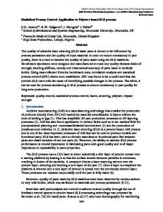
where Ni is the number of samples of each data matrix. After this linear transformation, the transformed data matrices, Y1 and Y2, have the same set of PCs and the PCs are reversely ordered. In other words, the most important correlation for one transformed data set Y1 is equivalent to the least important correlation for the other transformed data set Y2, and vice versa. An illustrative example is shown in Fig. 1.
Fig. 1. Transformation of data sets Xi (left) into Yi (right) for evaluating the dissimilarity.
Fig. 2. Methodology for MS-PCA.
177
The following dissimilarity index D was defined for evaluating the dissimilarity of data sets. 4 P D= % (lj − 0.5)2 (4) Pj = 1 Here, P is the number of variables and lj denotes the eigenvalues of the covariance matrix of the transformed data matrix. When data sets are quite similar to each other, the eigenvalues lj must be near 0.5. On the other hand, when data sets are quite different from each other, the largest and the smallest eigenvalues should be near 1 and 0, respectively. The index D changes between 0 and 1. When two data sets are similar to each other, D must be near 0. On the contrary, D should be near 1 when data sets are quite different from each other. For applying DISSIM, a reference data set and a control limit must be determined. The following procedure is adopted. 1. Acquire time-series data when a process is operated under a normal condition, and normalize the data. 2. Determine the size of time-window, w. Generate data sets with w samples from the data by moving the time-window. Then, select a reference data set from the data sets. 3. Calculate the index D, and determine the control limit. For on-line monitoring, the data matrix representing a current operating condition is updated by moving the time-window and scaled by using the mean and the variance obtained at step 1. Then, the index D is calculated.
2.3. Monitoring with multiscale PCA MS-PCA combines the ability of PCA to extract the relationship between variables and decorrelate the cross-correlation with the ability of wavelets to separate deterministic features from stochastic processes and approximately decorrelate the autocorrelation among the measurements. The steps in the MS-PCA methodology proposed by Bakshi (1998) for the process monitoring purpose are shown in Fig. 2, and the following procedure is adopted. 1. Acquire time-series data when a process is operated under a normal condition, and normalize the data. 2. Compute wavelet decomposition for each column in the data matrix, and generate L wavelet coefficient matrices, GjX { j= 1, …, L}, and one scaling function coefficient matrix, HLX. Here, L is the number of scales to be considered, Gi and HL represent filters, and X is the data matrix. 3. Apply PCA to the wavelet and the scaling function coefficient matrices, select an appropriate number of PCs, and determine control limits on the monitored indexes, T 2 and Q, at each scale.
M. Kano et al. / Computers and Chemical Engineering 24 (2000) 175–181
178 Table 1 Process disturbances Case 1 2 3 4 5 6 7 8 9 10 11 12 13 14 15 16–20
Disturbance
Type
A/C feed ratio B component D feed temp. Reactor cooling water (RCW) inlet temp. Condenser cooling water (CCW) inlet temp. A feed loss C header pressure loss A, B, C feed component D feed temp. C feed temp. RCW inlet temp. CCW inlet temp. Reaction kinetics RCW valve CCW valve Unknown
Step Step Step Step
The MS-PCA eliminates false alarms after process returns to normal operation through the steps of selecting scales that indicate significant events, reconstructing the measurements, and computing T 2 and Q of the reconstructed measurements. In addition, it should be noted that the control limits calculated at step 5 depend on the selection of scales used for the reconstruction.
Step Step Step Random Random Random Random Random Slow drift Sticking Sticking Unknown
3. Application In this section, several monitoring methods, including univariate SPC (USPC), conventional MSPC (cMSPC), MPCA, DISSIM, and MS-PCA, are applied to the monitoring problem of the Tennessee Eastman process.
3.1. Tennessee Eastman process The simulator of the Tennessee Eastman process was developed by Downs and Vogel (1993). The process consists of a reactor/separator/recycle arrangement involving two simultaneous gas–liquid exothermic reactions and two additional byproduct reactions, and it has 12 manipulated variables and 41 measurements. The simulator includes a set of programmed disturbances listed in Table 1. The control system utilized for dynamic simulations is the decentralized PID control system proposed by McAvoy and Ye (1994), which is shown in Fig. 3. The sampling interval was set to be at 3 min.
3.2. Settings for monitoring
Fig. 3. Decentralized control system of the Tennessee Eastman process.
4. Reconstruct the approximated data matrix from the coefficients at the selected scales. There are 2L + 1 combinations for selecting scales. 5. Apply PCA to the reconstructed data matrix, select appropriate number of PCs, and determine control limits on the monitored indexes, T 2 and Q. For on-line monitoring, current measurements are scaled by using the mean and the variance obtained at step 1, and then the measurements are filtered for calculating wavelet and scaling function coefficients. The indexes, T 2 and Q, of coefficients at the current time are calculated at each scale. The measurements are reconstructed from the coefficients at the selected scales where one of the current indexes violates the control limit. Finally, T 2 and Q of the reconstructed measurements are calculated.
The control limits of all indexes are determined so that the number of samples outside the control limits is 1% of the entire samples while the process is operated under a normal condition. On the basis of these control limits, the following steps evaluate all monitoring methods. 1. Each monitoring method is applied to faulty data, and each index is calculated. 2. For the data obtained after the occurrence of an error, the percentage of the samples outside the control limit is calculated in each simulation. Then, the mean of those percentages of ten different simulations is calculated in each case. Since each control limit is determined so that it represents 99% confidence limit, a monitoring method is regarded as successful in detecting the event if the mean calculated in step 2 is considerably higher than 1%. The mean gives a measure for evaluating the reliability of each index. It should be noted that the reliability depends on the number of samples. Hundred samples are used here for calculating the reliability.
M. Kano et al. / Computers and Chemical Engineering 24 (2000) 175–181 Table 2 Reliability (%) of MPCA Case
3
9
11
14
Index A1 A2 A3 A1–5 A1–10 A1–11 A1–12
41.6 39.3 2.4 2.1 2.6 40.9 0.0
34.6 29.1 1.6 2.3 0.5 40.4 0.0
3.0 6.3 1.3 1.7 2.6 71.5 0.1
85.7 85.4 1.3 1.9 3.7 97.6 0.0
A total of 16 variables, which are on-line measured process variables excluding manipulated variables, are used as monitored variables.
3.3. Results Several disturbances can easily be detected by using USPC. In other words, several disturbances can be detected immediately by monitoring each measured variable independently. For example, the reliability of USPC reached 99.2 and 95.5% in Case 1 and 2, respectively. It is very easy to detect such disturbances by using other monitoring methods. In the present study, disturbances, which are relatively difficult to detect by using USPC, are investigated. When utilizing cMSPC, the number of PCs must be determined. The number of PCs was set at 11, since the best performance was obtained at that number. When utilizing MPCA, the number of PCs and the size of time-window must be selected. For obtaining reliable PCs representing the operating condition at each step, a sufficient number of samples need to be used. On the other hand, use of an excessively large time-window can result in the reduced speed of detecting changes in the operating condition. From the results of having tried several different sizes of time-window, the size was set at 100 steps when each PC was monitored independently, and the size was set at 300 steps when the subspace spanned by several PCs was monitored.
179
The reliability of MPCA is strongly affected by the selection of PCs. A part of the monitoring results of MPCA are shown in Table 2. Here, A1 – k denotes the change of subspace spanned by the first k PCs. Although A1 and A2 are good indexes in Cases 3, 9, and 14, these indexes cannot detect an abnormal operating condition in Case 11. In Case 11, the subspace spanned by the first 11 PCs should be monitored. In other cases, A1 – 11 is the best or as good as the other indexes. It should be noted that the reliability of A1 – 11 is much higher than that of A1 – 10 and A1 – 12. These drastic changes of the reliability seem to indicate that the first 11 PCs are important for capturing the operating condition of the process. This result agrees with the previous result of cMSPC, where the best performance was given by using 11 PCs. When utilizing DISSIM, the size of time-window must be determined by considering the trade-off between the stability of data distribution and the detection speed. The size was set at 300 steps. When utilizing MS-PCA, the number of scales and the number of PCs must be selected. The number of scales was set at three, and the number of PCs was 11. The monitoring results are summarized in Table 3. Here, the subscript k of T 2k and Qk denotes the number of PCs used for calculating T 2 and Q. As expected cMSPC could outperform USPC in all cases. Furthermore, the reliability of MPCA and that of DISSIM are considerably better than that of cMSPC in Cases 3, 9, 11, 14, 16, and 19. On the other hand, MS-PCA outperforms cMSPC in Cases 11, 14, 16, and 19. In other cases, the reliability of cMSPC and that of MSPCA are comparable to each other. Since the influence of disturbance in Case 3 can be easily reduced by the control system, the deterministic changes of the monitored variables are not significant. Therefore, it is difficult to detect the change of operating condition by cMSPC and MS-PCA. However, MPCA and DISSIM can detect the change. These results have clearly shown the advantage of MPCA and DISSIM over cMSPC.
Table 3 Comparison of monitoring methods by reliability (%) Case Method USPC CMSPC MPCA DISSIM MS-PCA
Index
T 211 Q11 A1 A1–11 D T 211 Q11
3
8
9
10
11
14
16
19
20
3.5 1.7 18.9 12.6 41.7 58.1 19.6 10.7
43.7 84.6 88.2 100.0 86.4 84.9 86.2 87.5
7.2 3.1 14.9 11.6 41.0 28.8 15.0 13.8
40.4 76.5 81.2 100.0 77.9 79.7 78.5 81.3
6.0 0.8 20.4 0.0 71.4 49.4 4.0 47.9
31.6 6.2 70.8 0.0 97.5 92.5 65.5 94.5
9.8 9.0 21.9 84.0 43.3 60.9 23.4 39.0
6.0 10.3 11.3 15.9 36.0 52.9 29.5 44.3
41.9 67.4 69.1 100.0 61.2 68.5 67.1 68.5
w
300 100 300
180
M. Kano et al. / Computers and Chemical Engineering 24 (2000) 175–181
The reliability of MS-PCA is considerably higher than that of cMSPC in Case 11. The advantage of MS-PCA over cMSPC can be realized by its smoothing effect. MS-PCA has such a smoothing effect because decomposed signals in different frequency ranges are monitored. Such a smoothing effect is a drawback as well as an advantage because the detection speed might be reduced. Since MPCA and DISSIM also have a smoothing effect, which is caused by the time-window used for applying PCA on-line, their detection speed might be reduced. However, the reliability of MPCA and DISSIM is considerably higher than that of cMSPC. From the experience of applying the advanced monitoring methods to several other systems, DISSIM is easier to handle than MPCA because the number of PCs does not have to be selected. The monitoring performance in this application might be improved by using manipulated variables and measurements obtained from product analyzers as monitored variables, or by applying a dynamic monitoring method (Kano et al., 2181).
4. Integration of monitoring methods The monitoring performance of MPCA and DISSIM is better than that of the cMSPC method in many situations. MPCA and DISSIM can detect the changes in the operating condition even when the variances of monitored variables are decreased, since these two methods monitor the correlation among process variables. On the other hand, MS-PCA can also outperform the cMSPC method. The advantage of MS-PCA comes from the fact that the decomposed signals at several different frequency ranges are monitored independently. Therefore, further improvement of the monitoring performance is expected by integrating MPCA or DISSIM with the multiscale method. In this section, MS-MPCA and MS-DISSIM are proposed. The monitoring procedure of MS-MPCA and MSDISSIM is the same as that of MS-PCA, except the steps PCA in Fig. 2 is replaced by MPCA or DISSIM and the indexes, T 2 and Q, are replaced by Ai or D. For example, for on-line monitoring by MS-DISSIM, normalized measurements are filtered for calculating wavelet and scaling function coefficients, and then the dissimilarity index D of coefficients at the current time is calculated at each scale. The measurements are reconstructed from the coefficients at the selected scales where the current index violates the control limit. Finally, D of the reconstructed measurements is calculated and compared with its control limit. The reliability of MS-MPCA and MS-DISSIM was comparable to that of MPCA and DISSIM. The effectiveness of integrating MPCA or DISSIM with the
multiscale method was not clear in this example. In another simulated example, however, the performance of MS-MPCA and MS-DISSIM was considerably higher than that of MPCA and DISSIM. It should be noted that the multiscale method is advantageous especially in detecting small changes in the operating condition.
5. Conclusion Several statistical process monitoring methods were analyzed using simulated data obtained from the Tennessee Eastman process. In this article, the results with only ten realizations are shown, and the results provide a rough idea of the relative performance of various methods. More extensive monte–carlo simulations with smaller examples have been completed to provide statistically significant comparison between various methods. The monitoring performance of MPCA and DISSIM is considerably better than that of the cMSPC method in many situations. MPCA and DISSIM can detect the changes in the operating condition even when the deterministic changes in the monitored variables are not significant and the variances are not increased, since these two methods monitor the correlation among process variables. On the other hand, MS-PCA can also outperform the cMSPC method. The advantage of MS-PCA comes from the fact that decomposed signals at several different frequency ranges are monitored independently. Since MPCA and DISSIM have a smoothing effect, which is caused by the time-window used for applying PCA on-line, these two methods suffer from the delay. However, it should be noted that the speed and the reliability of fault detection could be adjusted by changing the time-window size. The selection of an appropriate size of time-window is crucial for an effective functioning of MPCA and DISSIM. Furthermore, MS-MPCA and MS-DISSIM can be used for combining the advantage of MPCA or DISSIM over cMSPC with that of MS-PCA.
Acknowledgements The authors gratefully acknowledge the financial support from the Japan Society for the Promotion of Science (JSPS-RFTF96R14301).
References Bakshi, B. R. (1998). Multiscale PCA with application to multivariate statistical process monitoring. American Institute of Chemical Engineering Journal, 44, 1596 – 1610.
M. Kano et al. / Computers and Chemical Engineering 24 (2000) 175–181 Downs, J. J., & Vogel, E. F. (1993). A plant-wide industrial process control problem. Computers & Chemical Engineering, 17, 245 – 255. Dunia, R., Qin, S. J., Edgar, T. F., & McAvoy, T. J. (1996). Identification of faulty sensors using principal component analysis. American Institute of Chemical Engineering Journal, 42, 2797 – 2812. Fukunaga, K., & Koontz, W. L. G. (1970). Application of the Karhunen – Loeve wxpansion to feature selection and ordering. IEEE Transactions Computer, C-19, 311–318. Kano, M., Nagao, K., Ohno, H., Hasebe, S., & Hashimoto, I. (1999). New methods of process monitoring using principal component analysis. In: American institute of chemical engineering annual meeting, paper 224a. Dallas, TX. Kano, M., Nagao, K., Ohno, H., Hasebe, S., & Hashimoto, I. (2181). Dissimilarity of process data for statistical process monitoring. Preprint of IFAC symposium on ad6anced control of chemical processes (ADCHEM). Kresta, J. V., MacGregor, J. F., & Marlin, T. E. (1991). Multivariate statistical monitoring of process operating performance.
.
181
Canadian Journal of Chemical Engineering, 69, 35 – 47. MacGregor, J. F., Jaeckle, C., Kiparissides, C., & Koutoudi, M. (1994). Process monitoring and diagnosis by multiblock methods. American Institute of Chemical Engineering Journal, 40, 826 – 838. McAvoy, T. J., & Ye, N. (1994). Base control for the Tennessee Eastman problem. Computers & Chemical Engineering, 18, 383– 413. Nomikos, P., & MacGregor, J. F. (1994). Monitoring batch processes using multiway principal component analysis. American Institute of Chemical Engineering Journal, 40, 1361 – 1375. Qin, S.J., Li, W., & Yue, H.H. (1999). Recursive PCA for adaptive process monitoring. In: Proceedings of the IFAC world congress, (pp. 85 – 90). Beijng, People’s Republic of China. Wise, B. M., & Gallagher, N. B. (1996). The process chemometrics approach to process monitoring and fault detection. Journal of Process Control, 6, 329 – 348. Wold, S., Geladi, P., Esbesen, K., & Ohman, J. (1987). Multi-way principal components- and PLS-analysis. Journal of Chemometrics, 1, 41 – 56.