Statistical Learning Methods Applied to Process ...

Statistical Learning Methods Applied to Process Monitoring: An Overview and Perspective Maria Weese1, Waldyn Martinez2, Department of Information Systems and Analytics Miami University, Oxford, OH, USA ([email protected] [email protected])

Fadel M. Megahed3 Department of Industrial and Systems Engineering Auburn University, Auburn, AL, USA ([email protected])

L. Allison Jones-Farmer4 Department of Information Systems and Analytics Miami University, Oxford, OH, USA ([email protected])

Abstract The increasing availability of high volume, high velocity data sets, often containing variables of different data types, brings an increasing need for monitoring tools that are designed to handle these big data sets. While the research on multivariate statistical process monitoring tools is vast, the application of these tools for big data sets has received less attention. In this expository paper, we give an overview of the current state of data-driven multivariate statistical process monitoring methodology. We highlight some of the main directions involving statistical learning and dimension reduction techniques applied to control charts in research from supply chain, engineering, computer science and statistics. The goal of this paper is to bring into better focus some of the monitoring and surveillance methodology informed by datamining techniques that show promise for monitoring large and diverse data sets. We introduce an example using Wikipedia search information and illustrate a few of the complexities of applying the available methods to a high dimensional monitoring scenario. Throughout, we offer advice to practitioners and some suggestions for future research in this emerging area of research. Keywords: Control charts, ensembles, neural networks, regression, support vector machines, variable selection

1 Dr. Weese is an Assistant Professor of Analytics in the Farmer School of Business. She is a Senior Member of ASQ. Her email address is [email protected]. 2 Dr. Martinez is an Assistant Professor of Analytics in the Farmer School of Business. His email address is [email protected]. 3Dr. Megahed is an Assistant Professor of Industrial and Systems Engineering at Auburn University. He is a Member of the ASQ. His email address is: [email protected] 4 Dr. Jones-Farmer is a Professor and Van Andel Chair of Analytics in the Farmer School of Business. She is a Senior Member of ASQ. Her email address is [email protected].

1

1.

INTRODUCTION

Control charts were proposed by Walter A. Shewhart in the 1920s as a tool to distinguish between the inherent (common cause) variation within the process and variations due to unwanted process disruptions (special cause). Control charts can be used retrospectively, in Phase I, or prospectively, in Phase II. The goal of Phase I is to understand the sources of process variability, define the in-control state of the process, and determine an in-control reference sample to design a control chart for Phase II monitoring. See, e.g., Jones-Farmer et al. (2014b) or Chakraborti et al. (2008) for a review of Phase I control charts. In Phase II, the process is monitored for departures from the in-control state. The goal of Phase II is to detect such changes as quickly as possible.

From the 1920s to the present, there have been many

developments in control chart methodologies; however, the applications of these newer methods in practice are limited. For example, the website used by the American Society of Quality to explain control charts is limited to a discussion of the traditional Shewhart charts with 3 limits (Teague 2004). Our experience indicates that when control charts are applied in industry, the applications are typically limited to Shewhart-type charts and Shewhart-type charts with runs rules. Our view is supported by several other researchers in the field. For example, Crowder et al. (1997, p. 139) stated that “[t]here are few areas of statistical application with a wider gap between methodological development and application than is seen in SPC.” Woodall (2000, p. 346) agreed by stating that “another unfortunate fact is that some useful advances in control charting methods have not had a sufficient impact in practice.” More recently, in his Youden Memorial Address, Vijay Nair stated that “there are far too many papers developing yet another charting procedure without considering whether the problem is important and whether the method can be actually used” (Nair, 2008). We believe that this issue remains valid, and it is a primary motivator for this paper. The goal of this paper is to bring to better focus some of the methods that rely on statistical learning and/or dimension reduction methods that show promise for monitoring large and diverse data sets. These large data sets, often termed big data, typically require more advanced statistical methods and often more

2

computing power than smaller, more manageable data sets. Unlike the origins of statistical monitoring, these applications are not limited to manufacturing, but also include opportunities in several application areas including social media, gaming, travel, insurance, healthcare, utility demand, and others (e.g., see Ning and Tsung 2010). The size of the data sets in these application areas is difficult to quantify and vary considerably by industry and application. Further, many of the methods we discuss are yet to be applied to data that would be considered big data relative to what is observed in industry. For example, Wal-Mart, the leading U.S. discount retailer, processes more than 1 million customer transactions per hour, resulting in databases estimated to be in the magnitude of 2,500 terabytes ("Data, Data Everywhere" 2010). In light of this, we consider methods that have been developed for larger and more diverse data sets than those typically considered in the statistical process control (SPC) literature and consider the potential scalability of these methods. We do not provide an extensive review of all papers that use statistical learning and/or dimension reduction methods along with control charts, but highlight the basic directions of this research. Our paper is focused, specifically, on how statistical learning methods have been used in developing SPC charts. Because the literature describing these methods has developed in a number of different research areas (e.g., manufacturing, operations management, statistics, and process control), SPC researchers may be unfamiliar with the developments in some of these other fields. Thus, our goal is to summarize the main research directions in several areas applying statistical learning to control charts in such a way that researchers and practitioners from different fields can understand, apply, and extend these methods for monitoring larger and more diverse data. There have been some focused reviews on data mining applications in manufacturing and quality control, and we discuss these in the appropriate sections of our paper. For example, Choudhardy et al. (2009) gave a high level overview of data mining methods used in manufacturing, but only briefly mentioned quality control applications. We assume that the reader is somewhat familiar with the basic concepts behind the construction and use of control charts (for detailed introductions, see Woodall and Adams 1998, Wheeler and Chambers 3

2010, Montgomery 2013). On the other hand, it is assumed that the reader is somewhat unfamiliar with statistical learning methods. Accordingly, in Section 2, we define our view of the term big data and provide some background information and references on several fundamental statistical learning methods. In Sections 3 and 4, we discuss the application of unsupervised learning and supervised learning methods, respectively, to process monitoring.

Throughout each section we review major

research streams, discuss how these methods can be used in big data settings, and offer some advice for practitioners, as well as suggestions for future research. In Section 5, we give an example related to monitoring Wikipedia search data to illustrate some of the complexities of applying control charts to high-dimensional data. Finally, in Section 6, we provide our concluding remarks.

2.

BACKGROUND INFORMATION

Big Data The term big data is used to describe large, diverse, complex, and/or longitudinal data sets that are generated from a variety of equipment, sensors, and/or computer-based transactions. Big data is often distinguished from other data by the 3V’s, the volume, variety, and/or velocity (Megahed and JonesFarmer 2015). Other important characteristics often associated with big data are veracity and value, but these are important characteristics for all data, not just big data (Jones-Farmer et al. 2014a). The methods associated with the analysis of big data are important for analyzing high volume, varied, high velocity process data.

While many of these methods have been used in the practice of process

monitoring for years (e.g. dimension reduction and regression-based methods), other methods originate from the fields of machine learning or statistical learning and are less familiar to researchers and practitioners in SPC. Many of these methods have foundations in data-driven (as opposed to modeldriven) analysis and may require a paradigm shift for many in SPC research and in practice. Nonetheless, there is much that can be learned in the field of SPC from the methods that have been developed for use in solving similar big data problems in other domains.

4

Statistical Learning Methods Statistical learning techniques have become very popular in the last two decades due to their versatility and power.

James et al. (2013) refer to statistical learning as a vast set of tools for

understanding data. These tools can be broadly classified as supervised or unsupervised learning. Supervised learning refers to inferring a mapping between a set of input variables x  {x1, x2 ,, x p } and an output variable y, given a training sample S   x1 , y1  , ,  xn , yn  of data pairs generated according to an unknown distribution Pxy with density𝑝(𝒙, 𝑦). The main goal of supervised learning is to estimate a function 𝐻: 𝕏 → 𝑌 such that 𝐻 will correctly classify unseen examples (𝒙𝒊 , 𝑦𝑖 ). The function is selected such that the generalization error 𝑅[𝐻] (also called the expected risk of the function) is minimized: 𝑅[𝐻] = ∫ 𝑔(𝑦, 𝐻(𝒙))𝑑𝑝(𝒙, 𝑦), where 𝑔(𝑦, 𝐻(𝒙)) is a suitable loss function.

(1)

One of the most common supervised learning

methodologies is least squares regression, where H is linear in its parameters and the generalization error is the sum of the squared model errors. Other common examples of supervised learning methods include logistic regression, artificial neural networks (ANNs), support vector machines (SVMs), and decision trees (DTs). In some situations, several supervised learning models can be combined to obtain better predictive performance than one could obtain from fitting a single model. Algorithmically combining multiple models together to improve model performance is commonly referred to as ensemble modeling. Ensemble models are often used to combine learning models such as decision trees that are considered to be weak on their own, but tend to be quite powerful when multiple trees are combined into a classifier. Boosting (Schapire 1990) refers to a family of methods that combine sequences of individual classifiers into highly accurate ensembles. AdaBoost (Freund and Schapire 1995) and gradient boosting (Friedman 2001) are two common boosting algorithms in which each subsequent model is trained to emphasize the cases that were misclassified from the previous modeling instance. Other ensemble approaches include

5

random forests (Breiman 2001a) and bagging (Breiman 1996). For an in-depth treatment of ensemble modeling, the reader is referred to Hastie et al. (2009, p. 605-624). Unsupervised learning describes an area of statistical learning that does not benefit from the availability of an outcome variable. The goal of unsupervised learning is to develop a framework or understand a pattern in the structure of the input variables{𝑥1 , 𝑥2 , … , 𝑥𝑝 }. Examples of unsupervised learning methods include cluster analysis, principal components analysis (PCA), latent variable methods, and mixture modeling. The choice of which statistical learning method to use often depends on the structure of the data. For example, some methods perform better when the input variables within x are scaled to a similar range, others perform poorly when the variables within x are highly redundant/correlated. Often, some form of data preprocessing is required prior to using statistical learning methods. There are some models (e.g. SVMs, neural networks, mixture models) that may be used in either a supervised or unsupervised way. Although we chose the broad classification of supervised vs. unsupervised learning methods to organize our paper, we readily admit that the distinction for particular applications of learning methods to statistical monitoring is often unclear, even within certain methodological papers. Statistical monitoring methods have benefited from the use of statistical learning techniques, especially through the application of statistical learning and dimension reduction methods. For example, ANNs, inductive learning, SVMs and decision trees have all been suggested as methods to be used to build control charts for monitoring and/or pattern recognition. Unsupervised learning methods such as cluster analysis and kernel estimation have been suggested for Phase I analysis in both traditional and profile monitoring applications of control charts. Dimension reduction methods such as PCA and factor analysis have been widely applied to control charts, often in conjunction with other supervised and unsupervised methods. As statistical learning methods become more mainstream, newer methods such as ensemble models are being considered for application to control charts as well. In the next sections, we will discuss an overview of each of these areas (unsupervised vs. supervised learning) as they have been applied to process monitoring. 6

3.

UNSUPERVISED LEARNING APPROACHES TO PROCESS MONITORING

Unsupervised learning methods are applicable when little is known about the process, and there is no information given as to what constitutes an out-of-control event. This makes unsupervised learning methods particularly applicable in Phase I of process monitoring. Jones-Farmer et al. (2014b) discussed some Phase I applications of unsupervised learning methods. In this section, we consider two broad classes of unsupervised learning methods: dimension reduction methods, and cluster and one-class classification methods. Although we realize that there is a difference between clustering methods and one-class classification methods, both unsupervised clustering and one-class classification methods are applied using a very similar framework in process monitoring. Dimension Reduction Methods In traditional statistical analyses, an observation typically refers to a certain phenomenon (e.g. a participant in a medical study) and we have a vector of values on several variables of interest (e.g. age, gender, weight, height, etc.). In such analyses, the assumption is that the number of observations, n, is much larger than the number of variables, p. However, in the age of big data, there has been an exponential increase in the number of variables, and more importantly their types. In a medical study, for example, the variables collected on the participant are often more complex, and can now include electromyography (EMG) signals, oxygen in-take profile, and medical images or movies, which make the number of dimensions associated with a single patient in the thousands or even millions. In this example, n, the number of patients, is likely to be much smaller than p, the number of variables. Sall (2013) referred to this phenomenon as wide data (as opposed to tall data). There are several approaches to reducing high-dimensional problems to lower-dimensional representations. Generally speaking these approaches can be classified into two main groups. In the first group, the focus is on selecting a subset of important variables, k, and ignoring the remaining not so important p – k variables. A classic example of this group in statistics involves the choice of predictors through variable selection methods in regression. The second group involves projecting the original set of variables into a lower dimensional subspace. Principal components analysis (PCA), partial least 7

squares (PLS), and factor analysis (FA) are all examples of such approaches. In this section, we consider some recent developments that are relevant to both Phase I and Phase II applications of control charts. The reader should note that, throughout this section, we use variables to denote the original/raw input variables and features to denote latent variables that are constructed from the input variables. Prior to explaining the process monitoring applications related to the two main areas of dimension reduction, it is important to note that the choice of whether the dimension should be reduced based on selecting a subset of variables or projection to a lower dimension is application dependent. In certain applications, it may be more meaningful to maintain a subset of the original variables based on some ranking criterion if this will facilitate the monitoring, diagnosis, and decision-making. If there is no need to maintain that original form of the variables, projection (or feature extraction) methods may be more suitable. Guyon and Elisseeff (2003) have constructed a heuristic-based checklist which summarizes the different steps that may be needed to approach feature selection problems. There are several streams of SPC research that discard the original set of variables (e.g. profile monitoring, risk-adjusted control charts, and much of the image monitoring literature). The distinction between whether the deployed method selected a subset of the variables or extracted features from these variables is often not clear. Variable Selection Approaches Applied to Process Monitoring. There is an increasing number of applications where there is a need to monitor high dimensional process data. In such applications, selecting a subset of “the most important” quality characteristics from the data may be sufficient for process monitoring.

Wang and Jiang (2009) suggested that the number of simultaneously shifted

variables is typically small in practice, and it would be both more beneficial and practical to reduce the monitoring to a smaller subset of variables that are responsible for the out-of-control conditions. Since the shifted variables are unknown in advance, Wang and Jiang (2009) proposed a procedure that combines a forward selection methods with multivariate control charting.

Zou and Qiu (2009)

investigated the use of the least absolute shrinkage and selection operator (LASSO) variable selection technique (Tibshirani 1996) to create a multivariate test statistic and integrated this statistic with a multivariate EWMA control chart. Capizzi and Masarotto (2011, 2013) recommended using Least Angle 8

Regression (LAR) (Efron et al. 2004) with a multivariate EWMA chart. LASSO and LAR for variable selection in multivariate SPC have also been suggested for profile monitoring (Zou et al. 2012), diagnosing process changes (Zou et al. 2011), and monitoring for changes in the covariance matrix (Maboudou-Tchao and Diawara 2013). From our perspective, the use of variable selection methods applied to the multivariate monitoring problem can be an efficient approach, but should be applied with caution. For example, one or more of the statistically “not so important variables” may suddenly become very important in a high velocity situation, and if eliminated, this change may go undetected. We recommend supplementing these approaches with expert knowledge on the process data, and suggest that users continuously monitor the goodness-of-fit of their models. A significant change in a measure of the goodness-of-fit may be an indicator of an out-of-control condition. The interested reader should refer to the discussion of the Qstatistic below for an example of how a similar problem is handled in chemometrics. Projection and Feature Extraction Methods Applied to Process Monitoring. The use of projection techniques and/or extracting features from the p-dimensional dataset has been implemented since the late 1980s in chemometrics (Wise et al. 1988, Wise and Ricker 1989, Kresta et al. 1991).

In these

applications, the dimension of the data is often reduced based on a model from PCA or PLS (Kourti and MacGregor 1995, MacGregor and Kourti 1995, Ferrer 2014).

The resultant components are then

monitored using a multivariate control chart such as the Hotelling’s T2 chart. Recently, the use of PCA, PLS, and their extensions with control charts have been applied to a number of different high dimensional domains.

For example, Megahed et al. (2011) presented a

discussion of the use of projection methods with control charts in the context of multivariate image analysis. Gronskyte et al. (2013) extended the use of PCA and the Hotelling T2 control chart to monitor the motion of pigs through video sequences. Yan et al. (2014) modeled the high-dimensional structure of image data with tensors and employed low-rank tensor decomposition techniques, including several extensions of PCA and a Tensor Rank-One Decomposition approach, to extract important features that are monitored using multivariate control charts. While these recent examples have all been in the 9

image/video monitoring domain, these approaches are highly effective in other domains of SPC. The reader is referred to Colosimo and Pacella (2007) for an example of using PCA in the context of functional data analysis, where PCA is used to identify systematic patterns in roundness profiles of manufactured parts. Two important points should be made based on the use of PCA/PLS with multivariate control charts. First, it is possible to move from the projection space back to the original data space. The second, and perhaps more important point, is that in the chemometric approaches involving PCA, a control chart is applied to the squared prediction error (also known as the Q-statistic or SPE statistic) to ensure that the process variability is still well modeled by the maintained principal components. We believe that this is a very important step since it ensures that the assumption that no significant information is lost due to the projection is valid when an unknown out-of-control condition occurs. Projection methods such as PCA can also be very useful in generating additional knowledge about the process being studied. Woodall et al. (2004) noted that PCA can be very useful in understanding process variation, an important step needed prior to moving to Phase II monitoring. Wells et al. (2012) showed that PCA can be used to describe unique geometric variation modes occurring during automotive manufacturing. We see four primary benefits of using PCA-like methods with larger data sets. The use of PCA-like methods in process monitoring: 1) can improve the analysis by removing the influence of redundant and noisy variables; 2) can make data processing easier; 3) can help to improve the interpretation and visualization of larger data sets; and 4) can help the practitioner to discover and understand the correlation structure of the data through the investigation of the component scores. These are all important aspects when monitoring larger data sets. The reader is referred to the package bigpca (http://cran.r-project.org/web/packages/bigpca/bigpca.pdf)

in

the

statistical

software

R

for

implementations of PCA for massive datasets. Clustering/One-Class Classification Methods Clustering methods may be based on an a priori model, such as mixture modeling, or algorithmic methods like k-means or hierarchical agglomerative clustering.

The line between model-free and 10

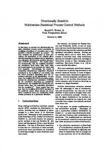
algorithmic clustering methods is not clear, as many algorithmic methods have been shown to be special cases of the model-based methods under certain model conditions. An excellent overview of clustering methods from a statistical perspective is given in Fraley and Raftery (2002). There are numerous clustering methods, and many of these have been applied to control charting. For example, in the chemical industry, model-based clustering methods such as mixture modeling have been used to define the in-control state of the process, or normal operating conditions. Mixture modeling is a method in which the distribution of independent variables is considered a mixture of two or more distributions that may differ in location, scale or correlation structure. Mixture models can be used alone (to create clusters) or in conjunction with a regression models where the clusters of independent variables predict a target variable. The use of model-based clustering with control charts usually combines a dimension reduction technique (e.g. PCA) with a mixture model approach. When estimating a mixture model, two sets of parameters are estimated: the distributional parameters (µ and  in the case of a Gaussian mixture); and mixture parameters that give the fraction of observations in each cluster. The number of clusters is often determined according to some criterion, e.g., Bayesian Information Criterion (BIC). Nylund et al. (2007) and Tofighi and Enders (2008) discussed criteria for selecting the number of clusters in a mixture model. Once the number of clusters and the distributional and mixture parameters are estimated, this information is used to establish a control region for the normal operating conditions of the process. Figure 1, reprinted from Thissen et al. (2005), compares the control region for two bivariate data sets. The graphs on the left show the in-control regions established using a Hotelling’s T2 approach versus the graphs on the right which show the in-control regions established using the mixture modeling approach. The mixture modeling approach produces an irregular in-control region, whereas the T2 approach gives an elliptical region. Although Figure 1 is based on simulated data, in real applications, the existence of multiple clusters within a reference sample could be an indicator of an out-of-control situation. We caution practitioners to conduct a thorough Phase I analysis of the data to understand the sources of variability and potential clustering of observations. References for those interested in the use of model11

based clustering methods for defining the in-control state of a process include, e.g., Chen and Liu (1999), Doymaz et al. (2001), Choi et al. (2004), Thissen et al. (2005), Chen et al. (2006).

Figure 1. Reprinted from Thissen et al. (2005) with permission. A comparison of control regions defined using a T2 approach (left) and the mixture modeling approach (right) for two different data sets (one data set per row). Similar to the model-based clustering methods, the one-class classification (OCC) approaches to process monitoring reframe the monitoring problem into a classification problem that classifies observations as either in- or out of control. This stream of research began with the introduction of the kchart (Sun and Tsung 2003). The k-chart is a control chart based on the support vector data description (Tax and Duin 1999, 2004) and designed for non-normal process data. Support vector data description (SVDD) is an unsupervised application of support vectors originally applied to machine fault diagnosis (Tax et al. 1999, Ypma et al. 1999). “The main idea of SVDD is to envelop the samples within a highdimensional space with the volume as small as possible” (Sun and Tsung 2003, p. 2979). Support vector methods use hyperplanes to divide multidimensional data into groups or classes. When hyperplanes are used to separate the data into classes, several difficult-to-classify observations will lie close to the separating planes.

These difficult-to-classify points, known as support vectors, are influential in

determining the separating hyperplane for correctly classifying observations.

The selection of the

separating hyperplanes can be determined based on the number of support vectors (influential observations) as well as the number of misclassified observations in the training sample. When a training sample is available, support vector methods allow for some degree of misclassification in order to obtain 12

a solution that is more robust to individual observations. Most applications of support vectors to process monitoring that we found used unsupervised support vector methods (e.g., SVDD) as an OCC to classify observations as either in- or out-of-control. The shape of the boundary determined using the SVDD method differs based on the different types of kernel functions used. Kernel functions used in support vector machines allow the user to implement a nonlinear boundary to separate the two classes of data (see pages 93-121 in Cristianini and Shawe-Taylor 2000). Figure 2 compares two kinds of boundaries for enclosing the data. The first boundary is based on a fitting a hypersphere and the second is based on SVDD.

Figure 2: Comparison of two kind of boundaries: hypersphere (left) and support vectors (right). Figure is from Sun and Tsung (2003). Reprinted with permission. The kernel distance-based control chart, k-chart, proposed by Sun and Tsung (2003) and updated by Ning and Tsung (2013) is designed for non-normal process data. The distance between an observation and the kernel center is the monitoring statistic used in the k-chart. The boundary for the data represents the control limit which distinguishes in-control observations from potential out-of-control observations. Note that the right-hand boundary in Figure 2 is not a regular boundary and cannot be expressed in explicit mathematical terms. Instead the boundary is determined by the support vectors (observations nearest to boundary), which can be obtained through solving a quadratic optimization problem (Sun and Tsung 2003, see Equations 22-23). A practitioner can adjust the boundary limits by the window width of the Guassian kernel function and a constraint in the optimization. Or in other words, how tightly the boundary fits the sample data. Optimal determination of this boundary for use as a control limit is a topic open for future research and is discussed in Ning and Tsung (2013). Control charts based on SVDD have the advantage of only depending on the support vectors; therefore, they are applicable to large amounts of 13

process data and variables. For an industrial application of the k-chart, the reader is referred to Gani et al. (2011). Several different modifications to the k-chart have been proposed in the literature. For example, Kumar et al. (2006) and Camci et al. (2008) have proposed modifications to the k-chart by using robust SVM (RSVM) to establish the minimum volume and improve upon the sensitivity of SVM to outliers present in the reference sample. Liu and Wang (2014) have proposed an adaptive-kernel-based (AK) control chart to improve the sensitivity of the multivariate chart to small process shifts. In addition to SVDD, other OCC control charts include the K2 chart, based on the-nearest neighbors data description (kNNDD) algorithm (Sukchotrat et al. 2009, Kang and Kim 2011). A summary of the different variants of the OCC charts is presented in Table 1. For each chart, we include an original citation introducing or studying the methods, the motivation to introduce the new method, and the type of classification method used. We also include the basis for the control limit, and where applicable, we list the type and if a kernel method is employed, provide information as to whether the method was developed based on independent and identically distributed (i.i.d.) observations, and how the method handles misclassification errors.

Table 1: A Summary of the Different Variants of OCC charts. Chart Name

Motivation

Method

Control Limit

Kernel Method

Assumes i.i.d.

Misclassification Error

k-chart (Sun and Tsung 2003)

Eliminate underlying distributional assumptions for Multivariate SPC Reduce the sensitivity to outliers in the reference data and to reduce potential over-fitting issues that can arise with the k-chart Eliminate underlying distributional assumptions, requires only incontrol data, offers methods for selecting limits

SVDD

Kernel Radius

Yes

RSVM

Kernel Radius

Gives information on changes in error rates with different number of support vectors. Gives information on changes in error rates with different number of support vectors.

SVDD and Support Vector Representation and Discrimination Machine (SVRDM)

Kernel Radius

Gaussian radialbased function (RBF) Compared 4 methods and showed Gaussian RBF performed best Gaussian RBF

Robust k-chart (Kumar et al. 2006)

rk-chart (Camci et al. 2008)

Yes

Yes

Employed an iterative procedure based on the data and number of support vectors to balance Type I/Type II errors.

14

KNNDD/KNN/K2 chart (Sukchotrat et al. 2009)

based on Type I and Type II errors Computationally more efficient than k-chart methods

kNNDD

Bootstrap percentile procedure

None

K-means chart (Kang and Kim 2011)

More quickly detects small shifts in the mean vector than the kchart.

KMDD

Specified distance from the individual cluster center

None

AK-chart (Liu and Wang 2014)

More quickly detects small shifts in the mean vector than the kchart.

SVDD

Genetic algorithm to establish action and warning regions based on Variable Sampling Intervals

Gaussian RBF

Shown to have better performance than a T2 chart when data are non i.i.d. (Kim et al. 2010) Yes

Yes

Employed a bootstrap procedure based on process data to select a control limit with a specified misclassification rate. Used an iterative process to determine control limit with specified misclassification rate for differing number of clusters. Employed a genetic algorithm based on process data and number of support vectors to determine a control limit with a specified misclassification rate.

Note that all the methods summarized in Table 1 are reported to be robust to non-normality and can be applied in Phase II. Although it has been suggested that some of these methods apply to Phase I, it is not clear to us how well these methods will work in the Phase I context. The number of observations required to establish an in-control reference sample is unclear, and little advice is given as to how to obtain this reference sample. The performance of several of OCC control charts, including both the kchart and the K2 chart, has been compared by Tuerhong and Kim (2014) using the average run length (ARL) metric, and their results show that increasing the number of observations improves the performance of the all of the charts compared. In quality control applications, it is generally important to maintain the time ordering of the process observations. Because many clustering/OCC methods do not preserve the time order of the data, it may be difficult to interpret signals to potential out-of-control events. There are several applications of clustering methods that attempt to preserve the sequential nature of process observations. For example, Sullivan (2002) used a clustering method to detect multiple change-points in a univariate process and

15

Ghazanfari et al. (2008) introduced a clustering approach to identify a step-change in a Shewhart control chart. Zhang et al. (2010) introduced a time-based univariate clustering method for determining an incontrol baseline from a historical data stream. Zhang et al. (2010) used the idea of subsequence clustering, by clustering the relative frequency distribution of a moving sequence of observations. We should note that the use of subsequence clustering is controversial within the machine learning literature; thus, we recommend that practitioners consult Keogh and Lin (2005) prior to implementing this approach. Clustering methods that aim to preserve the time ordering of the data have also been applied to the problem of multivariate outlier detection in SPC. For example, Jobe and Pokojovy (2009) introduced a computer intensive multi-step clustering method for retrospective outlier detection in multivariate processes. Jobe and Pokojovy (2009) compared their method to the retrospective use of the T2 chart with robust estimators for the covariance matrix and showed that their method was equal to or better than the robust T2 approaches in most situations considered. Clustering methods have also been suggested for use in the Phase I analysis of profiles. Chen et al. (2015) suggested replacing the process observations with an estimated profile that is determined using a regression method. These profiles are then clustered, and the cluster containing more than half of the data is identified as the set of in-control profiles. Chen et al. (2014) also consider the use of cluster analysis with nonparametric profiles. The applications of clustering and one-class classification methods in quality control are diverse (see Ge et al. (2011), Grasso et al. (2015) and Gani and Liman (2013)), and there remain many opportunities for research in this area, particularly in Phase I applications. For example, a noteworthy feature of many big data sets is the variety of the data, which often contain a mix of continuous, discrete, and possibly categorical variables. Future research should investigate the use of clustering, classification, and mixture modeling approaches for the Phase I analysis of data with multiple data types. We note that there may be some limitations to these approaches such as requirements of very large sample sizes, or the failure to preserve time ordering. There are also opportunities to consider the application of time series clustering 16

method to the analysis of both univariate and multivariate data that occur in streams. Because preserving the time order of process data is often critical, these methods may show promise in both Phase I and Phase II applications. It should also be noted that most methods discussed in this section assumed that the data within the clusters or classes can be stored in memory.

This may not be feasible in big data applications.

Rajaraman et al. (2014, Chapter 12.3) provides an excellent introduction to SVMs, and how to develop a parallel implementation schema which is necessary when the observed data is too big to be stored/analyzed in memory. This requirement is somewhat limiting with standard desktop computers; however, such approaches can be implemented with cloud computing. Therefore, there are opportunities for exploring clustering algorithms that do not store the cluster’s entire data in memory and evaluate how their performance in SPC applications. See Zhang et al. (1996), Bradley et al. (1998), and Guha et al. (1998) for three highly-cited examples of clustering algorithms that are suitable for big data sets.

4.

SUPERVISED LEARNING METHODS

In this section, we discuss the use of supervised learning methods in SPC. First, we discuss the problem of using computational methods based on supervised learning to detect abnormal patterns on control charts. While the majority of the literature in this area pertains to univariate data (which is not big data, per se), we briefly discuss this work since the bulk of the application of DT, ANN, and SVM models in SPC has been in the control-chart pattern-recognition (CCPR) literature. After discussing CCPR methods, we discuss control charts based on single supervised learning methods. Finally, we highlight the few papers that investigated using ensemble methods in SPC. As in Section 3, we offer advice to practitioners and highlight areas for future work whenever possible. Control Chart Pattern Recognition CCPR has its origins in the early days of SPC, starting with the Western Electric run rules in 1956. Champ and Woodall (1987) evaluated control charts with supplemental runs rules and showed that these charts can have a high incidence of false alarms. Like the classical approach to CCPR, the recent research on this topic is dedicated to identifying and classifying out of control patterns such as trends, cyclical 17

patterns and specific types of process shifts. In the modern CCPR literature, a supervised learner is trained to recognize specific types of process changes. The input into the statistical learning methods may be raw variables or linear or nonlinear combinations of the raw variables (i.e. features). ANN or SVM learners are used most often due their strong predictive ability. However, ANN and SVM learners can be difficult to interpret; thus, DT methods have been suggested to provide the user with more interpretive models pertaining to process changes. Many of the CCPR methods begin by simulating a reference data set containing in-control and out-ofcontrol data. The in- and out-of-control data are labeled as such, and this label serves as the target or outcome variable for a statistical learner. A statistical learner (e.g. ANN) is trained to distinguish the incontrol from the out-of-control data. The model that is developed is then applied to future observations, and these observations are either classified as in- or out of control. There are many simple and complex variations of the CCPR approaches to process monitoring. Although much of the literature in this area has typically considered low dimensional data (e.g. Zorriassatine et al. (2003), Cheng and Cheng (2011)), several authors focused on higher dimensional data (e.g. Deng et al. (2012), Dávila et al. (2011)). Deng et al. (2012) provided an overview of the major developments in this area as it relates to statistical monitoring. Deng et al. (2012) also noted that a limitation in these methods is that, most of the time, the classifiers are trained once based on a single artificial data set. They recommend a dynamic approach where the classifier is retrained with each new observation, and a statistic such as the classification error rate or class-probability is monitored. Zorriassatine and Tannock (1998) and Psarakis (2011) reviewed the literature on the use of neural networks with control charts, and many of these papers focus on the CCPR problem. Hachicha and Ghorbel (2012) provided a comprehensive review and analysis of the CCPR literature from 1991 to 2010 and highlighted several open research questions within this field. Hachicha and Ghorbel (2012) classified 122 CCPR papers according to a detailed schema that includes, e.g., the data model assumptions, the types and number of patterns studied, whether real data or simulated data were evaluated, and the performance measures used. Interestingly, the majority of the papers they reviewed (61.47%) used an 18

ANN approach to pattern recognition. Their study revealed that only nine authors have published nearly half of the 122 CCPR papers reviewed. Additionally, only 16 out of the 122 papers reviewed considered multivariate processes, and only five out of the 122 papers evaluated involved applying the proposed method on real process data (Hachicha and Ghorbel 2012, p. 210-213). Woodall and Montgomery (2014) stated that “Despite the large number of papers on this topic [neural network control charts including those for CCPR] we have not seen much practical impact on SPC”. We believe that this lack of impact on the practice of SPC is due to several reasons. In our review of the CCPR literature, we did not find any references or discussion addressing the baseline operation of a process or a mention of a Phase I analysis. Little advice is given as to how to apply the methods in practice, including how to establish an in-control baseline sample, how large the reference sample should be for the method to work effectively, and how to distinguish among the many choices of ANN architectures. These gaps make it difficult to apply the CCPR methods in practice and provide ample opportunities for future research in the practical application of CCPR methods. More work is needed to determine if these methods are truly beneficial for monitoring high dimensional process data. Consideration needs to be given to the robustness of these methods to the baseline training sample, including the baseline sample size. Guidelines need to be developed for practitioners as to how to select among the many types of CCPR methods. Further, we recommend that researchers study the ability of the CCPR charts to detect changes other than those for which the learners were specifically trained. Regression-Based Methods One approach to reducing the dimensions of a data set is through the construction of an outcome variable (or a smaller set of new features) that “summarizes” the data contained within the original pvariate vector.

In addition to the unsupervised dimension reduction methods discussed earlier,

supervised learning methods can be used to achieve a similar goal. In the SPC literature, there are two main streams for dimension reduction using regression methods: profile monitoring and risk-adjusted control charts for monitoring health-care outcomes.

19

Profile Monitoring. Profile monitoring is used to describe monitoring applications when the quality of a process/product is characterized by a relationship between a response variable and one or more explanatory variables. At each time-point, the observed data can be explained by fitting a profile. This can be achieved through simple linear, nonlinear, or nonparametric methods. Also, wavelets may be used if the data is projected to a frequency domain. In such situations, instead of monitoring and maintaining the entire set of observations, it is sufficient to maintain/monitor the parameters of the fitted model. Thus, the number of dimensions is reduced significantly. Woodall and Montgomery (2014), Woodall et al. (2004) and Woodall (2007) provided detailed reviews on this topic, with explanations of several applications for using profile monitoring. Some applications in profile monitoring include highdimensional 2D images (Wang and Tsung 2005) and 3D surface scans (Wells et al. 2013). Recently, Dai et al. (2014) have proposed a method for monitoring profile trajectories based on a dynamic time warping alignment for monitoring ingot growth in semi-conductor manufacturing. We believe that the concept of profile trajectories can be extended to applications involving cyber-security, credit-card fraud, among other business transactions where an intervention may be needed prior to obtaining the full profile/signal. For a more detailed discussion on the statistical analyses of profile monitoring, we refer the reader to Noorossana et al. (2011) who provide a detailed overview and a discussion of research needs. Risk-Adjusted Control Charts. Risk-adjusted control charts have been recommended for monitoring post-treatment outcomes in healthcare (Steiner et al. 2000). Unlike many industrial processes, the monitoring of post treatment outcomes provides the additional challenge that patients are not homogeneous and can have different risks prior to treatment to the underlying health conditions. For this reason, statistical methods used to monitor post treatment outcomes involve some sort of risk adjustment. Steiner et al. (2000) recommend using logistic regression to compute the odds of death for an individual patient based on a score that considered the patient’s preoperative health. They further suggested using two CUSUM control charts that are designed to detect a doubling and a halving of the odds of deaths. There are several other control charts used for this problem. For detailed reviews, the reader is referred 20

to Grigg and Farewell (2004), Woodall (2006), and Steiner (2014). In addition, Steiner (2014) and Fogel et al. (2015) provide excellent discussions on future research needs in this area. Neural Networks Most applications of neural networks in control charting research are in the area of CCPR. In this subsection, we introduce a similar application where neural network models are used in the simultaneous detection and diagnosis of process faults. The main motivation behind these methods lies in attempting to bridge between SPC research (where the focus has been on detecting an out-of-control condition) and engineering practitioners (where fault detection represents the first aspect of process monitoring). Chiang et al. (2001) identified four different stages of (engineering) process monitoring. The first step involves fault detection, where a statistical approach determines whether a fault, an out-of-control condition, has occurred. The next step, fault identification, involves identifying the subset of input variables/features that are most relevant to diagnosing the fault. This is followed by fault diagnosis, where the root-cause of the observed fault is identified. The final stage involves process recovery, where the fault is fixed and the process is returned to its in-control condition. The methods described within this subsection attempt to assist practitioners with the identification and diagnosis aspects since quick detection without identification and diagnosis is not informative, especially since in many applications it is assumed that the process is stopped once a control chart signals until the underlying issue is identified and the process is recovered (Montgomery 2013). Due to their predictive properties, ANN models typically assist in both the fault detectionidentification stages of process monitoring. Venkatasubramanian et al. (2003) discussed the application of ANN models in a review of what they call “process history based methods” for simultaneously detecting and identifying a process problem. Since it is not our objective to repeat the references they have reviewed, we will only highlight two of their key observations: 1) ANN models trained on historical process data are “limited in the sense of generalization” due to the fact they are trained on a sample of data to recognize certain process changes; and 2) There have been very few published papers that consider the application of ANN models to real industrial processes. It is important to note that the 21

first observation holds true for all supervised learning methods and not just neural networks. As for the second observation, we assert that the lack of guidance for a practitioner on how to apply an ANN even on the most basic level, like how to choose a baseline sample, is likely the reason that these methods have not been widely used. In our experience, an understanding of the true root-cause of a fault is often difficult.

We attribute this to the complexity of most manufacturing processes and a lack of

understanding of mechanisms for fault propagation. Although most of the methods using ANN for fault detection and identification consider continuous data that is not correlated over time, there have been a few papers that considered autocorrelated processes and attribute data. For example, Chiu et al. (2003) used an ANN to detect shifts in an autocorrelated process and compare its ability to identify which observations cause the shift to that of a cumulative sum (CUSUM) and an X-bar chart. Niaki and Abbasi (2008) propose using ANN to detect and classify mean shifts in multi-attribute processes. They varied the counts as well as the proportions in different attributes and showed that the ANN is able to detect the shift quicker than a multi-attribute npchart (Mnp) while simultaneously identifying the cause of the shift. It is surprising that there is not more work that takes advantage of ANN’s ability to use either continuous or categorical data, as we did not find any mixed data applications in our search. Support Vector Methods Although we discussed the unsupervised use of support vectors in Section 3, there are some applications of supervised SVM approaches to process monitoring and fault detection that warrant mention. Recently, Zhang et al. (2015) recommended a robust framework for detecting location shifts in a multivariate process using a SVM combined with a multivariate exponentially weighted moving average (MEWMA) control chart. SVM has also been applied to batch process monitoring (Yao et al. 2014) and in the use of support vector regression (SVR) as a precursor to residual based multivariate cumulative sum (MCUSUM) chart for monitoring autocorrelated data (Issam and Mohamed 2008). Chongfuangprinya et al. (2011) recommended monitoring the predicted probability of class membership from an SVM using bootstrap control limits. An earlier application of SVM is given by Chin et. al. 22

(2010) where SVM is integrated with independent component analysis (ICA) to improve fault detection in autocorrelated processes. Cheng et al. (2011) used SVM and ANN to estimate the magnitude of the shift in the process mean as detected by a CUSUM chart. In addition to process monitoring and fault detection, SVM has been applied to fault identification, that is identifying the variable or groups of process variables that have changed, either in mean or covariance structure, leading to an out of control situation. Moguerza et al. (2007) used SVMs for profile monitoring. Mahadevan and Shah (2009) suggested using SVM and ANN as an alternative to the T2 and SPE charts for monitoring and using a residuals plot for fault identification. The authors use a one-class SVM plot for fault detection and SVM Recursive Feature Elimination for fault identification. They applied this technique to two case studies using real process data and show its superiority over conventional methods. Cheng and Cheng (2008) compared SVM and ANN for fault identification, where the fault is a shift in the process covariance, and found that SVM and ANN methods performed similarly. They recommended SVM because it requires fewer tuning parameters when compared to ANN. Chiang et. al. (2004) compared SVM to Fisher discriminant analysis using data from the Tennessee Eastman Simulator for fault identification. In this work, a genetic algorithm was used to select key variables prior to using the fault identification methods. It is also assumed that there is prior knowledge regarding which variables are at fault and the type of process behavior that was exhibited from this fault is known. Although they can be computationally burdensome, both supervised and unsupervised applications of SVM have potential in the future of SPC methods applied to big data. In particular, we see that SVM may hold promise in studying process data comprised of a variety of data types since SVM is capable of handling both categorical and continuous data simultaneously. Interestingly, almost all the uses of SVM applications we found in SPC considered continuous data. Ensemble Methods Ensemble methods can be considered as a composite classification model, made up of different classifiers. The individual classifiers vote, and a class label prediction is returned by the ensemble method. Ensemble methods are typically more accurate than their component classifiers (Han and 23

Kamber 2011, p. 377). The applications of ensemble methods in process monitoring are similar to the different supervised methods. Du and Xi (2011) developed an interesting approach for fault diagnosis in assembly systems that combine multivariate control charts, engineering knowledge, and ensemble methods. In a similar method, Alfaro et al. (2009) used a T2 control chart to detect an out-of-control signal and applied boosted DT models as an alternative to a single ANN to identify which of the variables caused the signal. Jianbo et al. (2009) used an ensemble of ANN models referred to as Discrete Partial Swarm Optimization (DPSOEN) which improves upon the use of a single ANN model. Similar work was done with an ensemble of SVM classifiers by Cheng and Lee (2012). Yu and Xi (2009) also use the DPSOEN algorithm applied to linear combinations of the data to simultaneously monitor and identify a fault in a multivariate process. In combined applications of fault detection-identification-diagnosis, Li et al. (2006) used random forests (see Breiman 2001a) to find the change point and identify the at fault variables in a highdimensional multivariate process and showed that this supervised learning method outperforms a multivariate exponentially weighted moving average control chart. Not only does this method show promise in the realm of big data, but it forgoes the usual distributional assumptions that can be troublesome with multivariate SPC methods. It should be noted that Li et al. (2006) considered the time order of the data, where as many of learning methods applied to process monitoring do not preserve the time ordering of the process data. Hwang et al. (2007) applied random forests and regularized least squares to identify a multivariate control region. While a control region as defined by a multivariate T2 chart has a set false alarm probability under multivariate normality, their work aimed to define a region with a set false alarm probability but without the burden of a distributional assumption. Recently, Hwang and Lee (2015) proposed a new approach using random forests with artificially shifted data to improve classification of failures in situations when failures occur rarely. The application of ensemble methods in SPC seems to show the most promise for the challenges in monitoring big data with differing variable types and large dimensions. In fact, a recent application of ensemble methods in public health surveillance by Dávila et al. (2014) illustrated the use of an ensemble 24

of decision trees to monitor counts (or rates) of a disease. This greatly improves upon current methods of public health surveillance which typically involve only low dimensional data and cannot take into account additional data such as demographic information.

5.

EXAMPLE

Although the methods we discussed above rely on statistical learning methods, many of these methods have not been applied (at least not in the literature) to large, high-dimensional data sets. The purpose of this example is to illustrate some of the complexities associated with monitoring big data. It is impossible to find a scenario that concisely presents all, or even several of the methods we describe above. Our intent is to simply give an example of one potential monitoring scenario and the strengths and limitations of applying one type of method we describe above. One way to understand public interest that is generated by the popular press is to consider monitoring social media (e.g. Twitter, Facebook, etc.) and/or data from web searches (e.g. Google, Yahoo, Wikipedia). In our example, we consider recently generated data from Wikipedia searches related to the National Football League (NFL). In particular, we developed a dictionary of the NFL team names, coaches, managers and all currently active players, as of 09/15/2014. We downloaded the number of Wikipedia searches per hour for all terms in our dictionary between 09/01/2014 00:00 UTC (Coordinated Universal Time) and 09/15/2014 17:00 UTC. We specifically chose this data because (1) it represents modern data streams that would be considered big data by many; and (2) the data are counts (not multivariate normal), contain many zero values, have a nested correlation structure, and contain evidence of some high-profile events that spurred intense public interest. The data used for our example was gathered from http://dumps.wikimedia.org/other/pagecounts-raw/ which contains the hourly number of hits on all Wikipedia pages. Every hour contains a compressed file of approximately 100MB and a week of data holds over 16GB. The data contains all traffic for the time period on over two-million Wikipedia pages. To keep to our hypothetical example (and reduce the computational burden) we consider Wikipedia hits on only those pages listed in our NFL dictionary, which reduces our dimension to 𝑝 = 1916 pages, including all active players, coaches, teams and 25

managers. Our data set considers a two week period beginning on 9/1/2014 and was chosen to include the first two weeks of the 2014 season. The first week is used to establish a baseline for monitoring, and the second week constitutes our monitored observations. In this example, a signal to a potential out-ofcontrol event is defined as an unusually high number of Wikipedia hits on a particular team, coach, manager, or player. There are a number of interesting challenges in this monitoring problem.

The scenario is a

surveillance exercise, where the process cannot be stopped and recalibrated once a signal is observed. Shmueli and Burkom (2010) discussed many of the statistical challenges in biosurveillance. In this application, the observed counts are cyclical, with the number of Wikipedia search hits declining late at night, and peaking at specific times, especially on game days during the season (see Figure 3). Further, the data observed on each of the p=1916 pages are zero-inflated counts that are autocorrelated, and also cross-correlated due to the natural nesting structure of players and coaches within teams.

These

correlations depend on the performance of the players, playing time, injuries, etc. (see, e.g., Figure 4). Further correlations exist between teams, especially those paired as opponents during a game (see, e.g., Figure 5). In our example, the number of variables (team names, coaches, managers, and players) is larger than the number of observations (hourly hits). All of these data characteristics are expected for this type of internet traffic data, but constitute a challenge in the application of statistical monitoring.

Figure 3: Wikipedia traffic on “New England Patriots” from 9/1/2014 to 9/5/2014 to illustrate cyclic behavior of the Wikipedia traffic flow.

26

Figure 4: Overlay of Wikipedia traffic of Tom Brady and the New England Patriots over the selected time period illustrating the highly correlated and nested structure of the Wikipedia data.

Figure 5: Wikipedia traffic on Green Bay Packers and Seattle Seahawks over the selected time period illustrating the correlation between teams in the NFL. We readily admit that certain events that “go viral” may not need a statistical method to detect a process anomaly. For example, consider the player, Adrian Peterson, who was indicted on a child abuse charges on September 12, 2014. Figure 6 shows a dramatic increase in the number of hits on Adrian Peterson’s Wikipedia page on September 12, 2014. This is not surprising, and the “signal” is apparent without the use of statistical limits. This approach to the retrospective identification of a signal assumes that one would know to monitor Adrian Peterson to begin with, and uses only this single data stream. In other words, hindsight is 20/20, or it is relatively easy to pinpoint an event that we know has already occurred. More interesting, however, is monitoring the entire set of p=1916 variables to determine if there is a change in Wikipedia interest in the larger set of NFL teams, coaches, managers and players.

27

Figure 6: Illustrating the Wikipedia traffic for Adrian Peterson over the selected time period and the spike on 9/12/2014 relating to the alleged child abuse. The first step in defining a monitoring scheme for this data set is to define an appropriate method. To do so, we use the process of elimination, to eliminate those approaches that are not applicable to our scenario. Though our literature search, we found no methods that applied to high-dimensional zeroinflated counts that are both auto-correlated and cross-correlated with a natural nesting structure. This problem does not have a target or outcome variable, so it falls naturally within the realm of unsupervised methods. Thus, we focus our attention on the methods discussed in Section 3. Although the number of variables (p=1916) is much larger than the number of available hourly Wikipedia hits(𝑛 = 354) we did not use a dimension reduction technique. Many dimension reduction methods are unstable in high dimensional scenarios, and the nested structure of this data may result in components or features that are not meaningful. One could make an argument to monitor features of the data that take into account the nested structure of the data (i.e. different divisions, teams, players, etc.), but methods for feature extraction in nested data have not been directly applied to statistical monitoring. Our purpose here is to illustrate the application of existing methods to a high-dimensional data. Thus, we consider unsupervised methods that do not require distributional assumptions. Although we recognize several limitations to this approach, we considered the K2 (kNN) chart, an OCC control chart, which requires less computational cost than the K-chart (see Sukchotrat et al., 2009), is more robust to the i.i.d assumption requirement (Kim et al., 2010), and is more suitable for this application. Because we have obvious cyclic autocorrelation in this data, we borrowed from the bio28

surveillance literature and used the residuals from Holt-Winters model lagged by 24 hours on each player with seasonal and trend component (see Shmueli and Fienberg 2006; Burkom et al. 2007). We then analyzed the multivariate data set containing the p=1916 sets of residuals using the K2 chart. The first 168 observations taken during the first week of the season were used to establish the baseline Phase I sample. The remaining 162 observations (note the residuals for the lagged 24 observations were not used) taken during the second week of the season are using for Phase II monitoring. Fig. 7 shows the Phase I and Phase II K2 charts. All the K2 chart computations were done on Matlab using the Protools package (Duin et al., 2007). When applying the K2 chart, the choice of k, the number of nearest neighbors, determines the plotted statistic, which is the mean of the squared distance between each observation and each of the k nearest neighbors in a reference sample. The control limit for the K2 chart is determined using the percentile bootstrap method, where the mean of the squared distances for each observation in the reference sample are bootstrapped, and the 1-α quantile of the bootstrapped distribution gives the control limit. Breunig et al. (2000) recommended a range of k between 10 and 50. In this example, the choice of k made little difference since there were a number of hours in the reference sample with no Wikipedia hits, and these observations formed the k nearest neighbors; thus, we selected k = 20, and α=0.01. As stated earlier, the literature we reviewed gives no guidance on proper Phase I analysis for process data such as this. Because of the similarities with biosurveillance, we consulted the recent review by Shmueli and Burkom (2010) who noted that Phase I implementation is extremely challenging in scenarios such as these due to the lack of sufficient Phase I data. In the circumstances of this example we believe it would be extremely difficult (if not impossible) to conduct a proper Phase I analysis; however, we did our best to comply with basic principles of Phase I. As such, we assume the process should be operating in a typical fashion, free from anomalies or unusual sources of variability. If anomalies or unusual sources of variability are present, these are removed only if an assignable cause can be identified. In the Phase I chart in Figure 6, we notice two signals of potential out-of-control events. Further investigation into these time periods reveals possible assignable causes (see Table 2). We did not remove these signals from our 29

analysis for two reasons: (1) We are not certain that these signals are anomalous to the process, thus we chose to leave them in the sample; and (2) Sukchotrat et al. (2009) did not discuss an iterative approach to the K2 chart, where assignable causes are removed and the limits recalculated. Because the K2 chart uses only a small subset of the Phase I data as nearest neighbors for computation of the chart statistic, the removal of out-of-control observations has no effect on the chart statistics in our example. However, removal of the out-of-control events would change the sample upon which the bootstrap limits are based. We explored removing these observations, and found only minimal changes in the control limits, thus we elected to leave these observations in the reference sample for calculation of the Phase II limits. Figure 7 also shows the Phase II application of the K2 chart, in which the k=20 nearest neighbors established in Phase I are used to determine the status of future observations. In Figure 7, we see a signal, and Table 2 gives two possible explanations for this signal.

Figure 7: Phase I and II K2 charts of the NFL Wikipedia data over the two week time period. Table 2: Summary of signals for Phase I and Phase II application of K2 chart to Wikipedia NFL player’s, coaches, and team’s page hits.

30

Date and Time of Signal

Possible Assignable Causes

Phase I

09/04/2014 20:00:00 UTC

Phase II

09/07/2014 17:00:00 UTC 09/09/2014 19:00:00 UTC

Packers vs. Seahawks game. Aaron Rodgers had a poor performance and Russell Wilson had a particularly good game. Sunday Football games LeSean McCoy was called out by a restaurant owner for leaving a $0.20 tip on $61.56 meal. This incident was highly publicized (see link 1, link 2 and link 3 for examples of media coverage). ESPN’s E:60 aired an episode on Marquise Goodwin and his sister Deja, born with cerebral palsy.

While not a perfect analysis, the use of the K2 chart in this example provides an example of the need for more research on data driven (as opposed to model-based) control charts (see Breiman (2001b) for an interesting discussion of model-based versus data-driven statistical models). The use of unsupervised learning methods may provide valuable information for very large and broadly defined “processes” involving organizations such as the NFL, separating common-cause variability in public or media interest from special cause events. Charts such as these may provide insight as to what constitutes an unusual event in a process involving high-dimensional, correlated data streams. There are many open research questions with the OCC control charts, and their performance has not been well-studied. This example is not intended to encompass all of the challenges present in big data monitoring, but serves as one example of a few of the complexities of this type of data.

6.

CONCLUDING REMARKS

We have given an overview of the main research streams that apply statistical learning methods to statistical process monitoring. Although many of these methods have not been directly studied using data sets that would be considered big data, some of these methods may be scalable to such problems. Our view is that there is a significant need for statistical monitoring of data streams and big data for detection of process changes as well as identifying the root-cause for these changes. The ability to gather observations instantaneously, often in real-time, results in observations possessing a high degree of autocorrelation. The effect of autocorrelation on traditional control charts has been studied by, e.g., Maragah and Woodall (1990), Alwan (1992), and Psarakis and Papaleonida (2007). Several authors have recommended statistical learning methods for monitoring autocorrelated data, 31

including Arkat et al. (2007), Isaam and Mohamad (2008), and Kim et al. (2012). Most of these methods apply a statistical learning method to the residuals of a time series model. There is not much literature on how to monitor autocorrelated data when the time series model is unknown; thus, we recommend more research in this area to further the development of monitoring and surveillance in high velocity data streams. Additionally, in traditional SPC applications, there are two often-made assumptions regarding the role of engineering/process knowledge: a) much process knowledge and understanding is needed in transitioning from Phase I and Phase II; and b) the identification and diagnosis of a process fault is primarily based on process knowledge informed by the output of control charting or other monitoring methodologies. As shown in the example, in big data sets, the retrospective analysis done in Phase I remains critical since it allows us to understand the behavior of the process being studied. Unlike in traditional applications, there are often no physical or engineering principles that can be used to understand this behavior. Accordingly, the goals of Phase I in big data applications include the typical goals of understanding process behavior, estimating the in-control parameter values needed for constructing Phase II methods as well as an increased emphasis on exploratory data analysis where statistical graphs and visual data mining approaches (see, e.g., Smith et al., 2014) can be used to provide insight into the behavior of the process. As for the diagnosis of signals (either in Phase I or II), it can be informed by the knowledge gained from the existing process data or from the fusion of data from multiple sources. Statistical learning methods have been suggested for identifying root causes for process changes, mostly in the field of engineering process control under the moniker “fault identification” or “fault diagnosis”. For example, Li et al. (2008) proposed a method to decompose the Hotelling’s T2 statistic based on a Bayesian network. Du et al. (2012) recommended classifying mean shifts from multivariate charts using a multi-class SVM. Kim et al. (2011) proposed a decomposition of Hotelling’s T2 chart using a one-class classification algorithm.

32

In addition to using analysis based only on the monitored variables, it may be necessary to incorporate data from other sources in order to properly identify the root-cause of a process signal (e.g., Hyniewiz (2015)). For example, the potential assignable causes showed in Table 2 have been determined from analyzing news articles around these time periods. If such articles had not been found, text analytics of the play-by-play descriptions on NFL.com (which can be easily done in the Python Programming Language with the package nflgame) can assist in understanding if the signal is related to a player’s performance in a NFL game. However, if both media sources and NFL.com do not indicate that there is an on-the-field or off-the-field issue that led to a signal, then one might speculate that the signal is caused by a cyber-attack on the Wikipedia website where web-crawlers are increasing the load on the Wikipedia servers. This determination may then be confirmed by examining the IP addresses for the visitors of the Wikipedia pages that led to a signal. From the above discussion, we see an important opportunity for researchers in both statistical learning and industrial statistics to refine existing methods and develop new methods to monitor multiple related-data streams (e.g. Twitter, Facebook, Google Search statistics and Wikipedia data) in big data applications. The fusion of information from these multiple data-streams may assist in increasing the veracity of the data, an important issue in big data surveillance as highlighted in Megahed and Jones-Farmer (2015). The benefits of merging data sources from multiple streams (with a discussion of statistical approaches for how to do it) is explained in more detail within the context of biosurveillance by Shmueli and Fienberg (2006, see Section 4 pp. 123-133). We also see tremendous opportunity for developments regarding how one establishes an in-control reference sample (Phase I) for multivariate processes, and especially for multivariate processes measured with mixed variable types. Further, we see the need for growth in the application of statistical learning methods to high-volume, high-dimensional, and high-velocity processes.

Because most of the

applications considered in the literature pertain to lower-dimensional data, the scalability of these monitoring methods in high dimensions is not fully understood. Lastly, most big process data sets have a complex structure, with distinct cyclic patterns of autocorrelation (day-of-week, time-of-day, etc.), are

33

derived from multiple streams, and often have some type of a hierarchical or nested structure. Monitoring this data with the existing techniques is challenging, and our experience suggests that the traditional model-based SPC methods are ill-suited to big data monitoring. The future of statistical monitoring in big data applications is likely to become more data driven as opposed to model driven and will rely more heavily on statistical and machine learning algorithms.

ACKNOWLEDGEMENTS This work was partially supported by an Amazon Web Services, Educational Grant to Auburn University. The authors would also like to thank Huw Smith and Jordan Huff, graduate students at Auburn University, for their assistance in developing a dictionary containing all names of NFL players (based on the Python nfldb package) and in extracting the relevant data from the Wikipedia Compressed (.gz) files.

REFERENCES Alfaro, E., Gamez, M., and Garcia, N. (2009), “A boosting approach for understanding out-of-control signals in multivariate control charts,” Journal of Production Research, 47, 6821-6831. Alwan, L.C. (1992), “Effects of Autocorrelation on Control Chart Performance,” Communication in Statistics –Theory and Methods, 21, 1025-1049. Arkat, J., Niaki, S.T.A, Abbasi, B.(2007), “Artificial Neural Networks in Applying MCUSUM Residuals Charts for AR(1) Processes,” Applied Mathematics and Computation, 189, 1889-1901. Bradley, P. S., Fayyad, U., and Reina, C. (1998), “Scaling Clustering Algorithms to Large Databases,” Proceedings of the 4th International. Conference on Knowledge Discovery and Data Mining (KDD’98), 9-15. Breiman, L. (1996), “Bagging Predictors,” Machine Learning, 24, 123-140. Breiman, L. (2001a), “Random Forests,” Machine Learning, 45, 5-32. Breiman, L. (2001b), “Statistical Modeling: The Two Cultures”, Statistical Science, 16, 199-231. Breunig, M.M., Kriegel, H.P., Ng, R.T. and Sander, J. (2000), “LOF: identifying density-based local outliers,” Proceedings of the ACM SIGMOD 2000 International Conference on Management of Data, 29, 93–104. Burkom, H.S., Murphy, S., and Shmueli, G. (2007), “Automated Time Series Forecasting for Biosurveillance,” Statistics in Medicine, 26, 4202-4218.

34

Camci, F., Chinnam, R.B., and Ellis, R.D. (2008), “Robust Kernel Distance Multivariate Control Chart Using Support Vector Principles,” International Journal of Production Research, 46, 5075-5095. Capizzi, G., and Masarotto, G. (2011), "A Least Angle Regression Control Chart for Multidimensional Data," Technometrics, 53, 285-296. Capizzi, G., and Masarotto, G. (2013), “Efficient Control Chart Calibration by Simulated Stochastic Approximation,” XIth International Workshop on Intelligent Statistical Quality Control. Chakraborti, S., Human, S. W., and Graham, M. A. (2008), “Phase I statistical process control charts: an overview and some results.” Quality Engineering, 21(1), 52-62. Champ, C. W., and, Woodall, W. H. (1987), “Exact Results for Shewhart Control Charts with Supplementary Runs Rules,” Technometrics, 29, 393-399. Chen, J. H., and Liu, J. L. (1999), “Mixture Principal Component Analysis Models for Process Monitoring,” Industrial & Engineering Chemistry Research, 38, 1478-1488. Chen, T., Morris, J., and Martin, E. (2006), “Probability Density Estimation Via an Infinite Gaussian Mixture Model: Application to Statistical Process Monitoring,” Journal of the Royal Statistical Society: Series C, 55, 699-715. Chen, Y., Birch, J. B., and Woodall, W. H. (2014), “A Phase I Cluster-Based Method for Analyzing Nonparametric Profiles,” Quality and Reliability Engineering International, DOI: 10.1002/qre.1700. Chen, Y., Birch, J. B., and Woodall, W. H. (2015), “Cluster-Based Profile Analysis in Phase I,” Journal of Quality Technology, 47, 14-29. Cheng, C. and Lee, H. (2012), “Identifying the out-of-control variables of multivariate control chart using ensemble SVM classifiers,” Journal of the Chinese Institute of Industrial Engineers, 5, 314-323. Cheng, C.S. and Cheng, H.P. (2008), “Identifying the source of variance shifts in the multivariate process using neural networks and support vector machines,” Expert Systems with Applications, 35, 198-206. Cheng, C. S., and Cheng, H. P. (2011), “Using Neural Networks to Detect the Bivariate Process Variance Shifts Pattern,” Computers & Industrial Engineering, 60, 269-278. Cheng, C., Chen, P., and Huang, K. (2011), “Estimating the Shift Size in the Process Mean with Support Vector Regression and Neural Networks,” Expert Systems with Applications 38, 10624-10630. Chiang, L. H., Braatz, R. D., and Russell, E. L. (2001), Fault Detection and Diagnosis in Industrial Systems, London, UK: Springer. Chiang, L., Kotanchek, M.E., and Kordon, A.K. (2004), “Fault Diagnosis Based on Fisher Discriminant Analysis and Support Vector Machines,” Computers and Chemical Engineering, 28, 1389-1401. Chin, H., Chen, C., and Long-Sheng, C. (2010), “Intelligent ICA-SVM fault detector for non-Gaussian multivariate process monitoring,” Expert Systems with Applications, 37, 3264-3273. Chiu, C. C., Shao, Y. J. E., Lee, T. S., and Lee, K. M. (2003), “Identification of Process Disturbance Using Spc/Epc and Neural Networks,” Journal of Intelligent Manufacturing, 14, 379-388. 35

Choi, S. W., Park, J. H., and Lee, I. B. (2004), “Process Monitoring Using a Gaussian Mixture Model Via Principal Component Analysis and Discriminant Analysis,” Computers & Chemical Engineering, 28, 1377-1387. Chongfuangprinya, P., Kim, S.B., Park, S.K., and Sukchotrat, T. (2011), “Integration of Support Vector Machines and Control Charts for Multivariate Process Monitoring,” Journal of Statistical Computation and Simulation, 81, 1157-1173. Choudhardy, A.K., Harding, J.A., and Tiwai, M.K. (2009), “Data Mining in Manufacturing: a Review Based on the Kind of Knowledge,” Journal of Intelligent Manufacturing, 20, 501-521. Colosimo, B. M., and Pacella, M. (2007), “On the Use of Principal Component Analysis to Identify Systematic Patterns in Roundness Profiles,” Quality and Reliability Engineering International, 23, 707725. Cristianini, N, and Shawe-Taylor, J. (2000), Support Vector Machines and other kernel-based learning methods. Cambridge, U.K.: Cambridge University Press. Crowder, S. V., Hawkins, D. M., Reynolds, M. R., and Yashchin, E. (1997), “Process Control and Statistical Inference,” Journal of Quality Technology, 29, 134-139. Dai, C., Wang, K., and Jin, R. (2014), “Monitoring Profile Trajectories with Dynamic Time Warping Alignment,” To appear in Quality and Reliability Engineering International. “Data, Data Everywhere,” (2010), The Economist, 394, 3-16. Retrieved August 27, 2014, from http://www.economist.com/node/15557443. Dávila, S., Runger, G., and Tuv, E. (2011), “High-Dimensional Surveillance,” in Artificial Neural Networks and Machine Learning – Icann 2011 (Vol. 6792), eds. T. Honkela, W. Duch, M. Girolami and S. Kaski, Springer Berlin Heidelberg, pp. 245-252. Dávila, S., Runger, G., and Tuv, E. (2014), “Public Health Surveillance with Ensemble-Based Supervised Learning,” IIE Transactions, 46, 770-789. Deng, H., Runger, G., and Tuv, E. (2012), “System Monitoring with Real-Time Contrasts,” Journal of Quality Technology, 44, 9-27. Doymaz, F., Chen, J., Romagnoli, J. A., and Palazoglu, A. (2001), “A Robust Strategy for Real-Time Process Monitoring,” Journal of Process Control, 11, 343-359. Du, S., and Xi, L. (2011), “Fault Diagnosis in Assembly Processes Based on Engineering-Driven Rules and PSOSAENAalgorithm,” Computers & Industrial Engineering, 60(1), 77-88. Du, Shichang, Jun Lv, and Lifeng Xi (2012), "On-line Classifying Process Mean Shifts in Multivariate Control Charts Based on Multiclass Support Vector Machines." International Journal of Production Research 50, 6288-6310. Duin, R.P.W., Juszczak, P., Paclik, P., Pekhalska, E., de Ridder, D., Tax, D.M.J., and Verzakov, S. (2007), “PRTools4.1, A Matlab Toolbox for Pattern Recognition”, Delft University of Technology.

36

Efron, B., Hastie, T., Johnstone, I., and Tibshirani, R. (2004), “Least Angle Regression,” The Annals of Statistics, 32, 407-499. Ferrer, A. (2014), “Latent Structures-Based Multivariate Statistical Process Control: A Paradigm Shift,” Quality Engineering, 26, 72-91. Fogel, S.L., Steiner, S.H. and Woodall, W.H. (2015), “The Monitoring and Improvement of Surgical Outcome Quality,” To appear in Journal of Quality Technology. Fraley, C., and Raftery, A. E. (2002), “Model-Based Clustering, Discriminant Analysis, and Density Estimation,” Journal of the American Statistical Association, 97, 611-631. Freund, Y., and Schapire, R. (1995), “A Desicion-Theoretic Generalization of on-Line Learning and an Application to Boosting,” in Computational Learning Theory, 904, ed. P. Vitányi. Springer Berlin Heidelberg, 23-37. Friedman, J. H. (2001), “Greedy Function Approximation: A Gradient Boosting Machine,” Annals of Statistics, 29, 1189-1232. Gani, W., Taleb, H., and Liman, M. (2011), “An Assessment of the Kernel-distance-based Multivariate Control Chart through an Industrial Application,” Quality and Reliability Engineering International, 27, 391-401. Gani, W., and Liman, M. (2013), “Performance Evaluation of One-Class Classification-based Control Charts through and Industrial Application,” Quality and Reliability Engineering International, 29, 841854. Ge, Z., Gao, F. and Song, Z. (2011) “Batch Process Monitoring based on Support Vector Data Description Method,” Journal of Process Control, 21, 949-959. Ghazanfari, M., Alaeddini, A., Niaki, S. T. A., and Aryanezhad, M.-B. (2008), “A Clustering Approach to Identify the Time of a Step Change in Shewhart Control Charts,” Quality and Reliability Engineering International, 24, 765-778. Grigg, O., and Farewell, V. (2004), “An Overview of Risk‐Adjusted Charts,” Journal of the Royal Statistical Society: Series A, 167, 523-539. Grasso, M., Colosimo, B.M., Semeraro, Q. and Pacella, M. (2015), “A Comparison of Distribution-Free Multivariate SPC Methods for Multimode Data”, Quality and Reliablity Engineering International, 31, 75-76. Gronskyte, R., Kulahci, M., and Clemmensen, L. K. H. (2013), "Monitoring Motion of Pigs in Thermal Videos," Workshop on Farm Animal and Food Quality Imaging 2013, 31-36. Guha, S., Rastogi, R., and Shim, K. (1998), “Cure: An Efficient Clustering Algorithm for Large Databases,” Proceedings of the 1998 ACM SIGMOD international conference on Management of data, 73-84. Guyon, I., and Elisseeff, A. (2003), “An Introduction to Variable and Feature Selection,” Journal of Machine Learning Research, 3, 1157-1182.

37

Hachicha, W., and Ghorbel, A. (2012), “A Survey of Control-Chart Pattern-Recognition Literature (19912010) Based on a New Conceptual Classification Scheme,” Computers & Industrial Engineering, 63, 204-222. Han, J., and Kamber, M. (2011), Data Mining : Concepts and Techniques (3rd ed.), Burlington, MA: Elsevier. Hastie, T., Tibshirani, R., Friedman, J., Hastie, T., Friedman, J., and Tibshirani, R. (2009), The Elements of Statistical Learning, 2nd Edition. New York: Springer. Hyniewicz, O. (2015), SPC of Processes with Predicted Data: Application of the Data Mining Process. In S. Knoth & W. Schmid (eds.), Frontiers in Statistical Quality Control (219-235). Switzerland: Springer International Publishing. Hwang, W., and Lee, J.S. (2015), “Shifting Artificial Data to Detect System Failures,” International Transactions in Operational Research, 22, 363-378. Hwang, W., Runger, G. and Tuv, E. (2007), “Multivariate Statistical Process Control with Artificial Contrasts,” IIE Transactions, 39, 659-669. Issam, B.K. and Mohamed, L. (2008), “Support Vector Regression Based Residual MCUSUM Control Chart for Autocorrelated Process,” Applied Mathematics and Computation. 201, 565-574. James, G., Witten, D., Hastie, T., and Tibshirani, R. (2013), An Introduction to Statistical Learning with Applications in R, New York, NY: Springer. Jianbo, Y., Lifeng, X., Xiaojun, Zh. (2009), “Identifying Source(s) of Out-of-Control Signals in Multivariate Manufacturing Processes Using Selective Neural Network Ensemble,” Engineering Applications of Artificial Intelligence, 22, 141-152. Jobe, J. M., and Pokojovy, M. (2009), “A Multistep, Cluster-Based Multivariate Chart for Retrospective Monitoring of Individuals,” Journal of Quality Technology, 41, 323-339. Jones-Farmer, L. A., Ezell, J. D., and Hazen, B. T. (2014a), “Applying Control Chart Methods to Enhance Data Quality,” Technometrics, 56, 29-41. Jones-Farmer, L.A., Woodall, W.H., Steiner, S.H., and Champ, C.W. (2014b), “An Overview of Phase I Analysis for Process Improvement and Monitoring,” Journal of Quality Technology, 46, 265-280. Kang, J.H. and Kim, S.B. (2011), “Clutering-Algorithm-based Control Charts for Inhomogeneously Distributed TFT-LCD Processes,” International Journal of Production Research, 51, 5644-5657. Keogh, E., and Lin, J. (2005), "Clustering of Time-Series Subsequences Is Meaningless: Implications for Previous and Future Research," Knowledge and Information Systems, 8, 154-177. Kim, S.B., Jitpitaklert, W., Park, S.K., Hwang, S.J. (2012), Data Mining Model-Based Control Charts for Multivariate and Autocorrelated Processes, Expert Systems with Applications, 39 (2), 2073-2081. Kim, S.B., Sukchotrat, T., and Park, S.K. (2011), “A Nonparametric Fault Isolation Approach Through One-class Classification Algorithms,” IIE Transactions, 43, 505-517.

38

Kim, S.B., Weerawat, J., and Sukchotrat, T. (2010), “One-class classification-based control charts for monitoring autocorrelated multivariate processes,” Communications in Statistics-Simulation and Computation, 39, 461-474. Kourti, T., and MacGregor, J. F. (1995), “Process Analysis, Monitoring and Diagnosis, Using Multivariate Projection Methods,” Chemometrics and Intelligent Laboratory Systems, 28, 3-21. Kresta, J. V., MacGregor, J. F., and Marlin, T. E. (1991), “Multivariate Statistical Monitoring of Process Operating Performance,” The Canadian Journal of Chemical Engineering, 69, 35-47. Kumar, S., Choudhary, A.K., Kumar, M., Shankar, R. and Tiwari, M.K. (2006), “Kernel Distance-Based Support Vector Methods and its Application in Developing a robust K-chart,” International Journal of Production Research. 44, 77-76. Li, J., Jin, J., Shi, J. (2008), “Causation-based T2 Decomposition for Multivariate Process Monitoring and Diagnosis,” Journal of Quality Technology, 40, 46–58. Li, F., Runger, G.C., and Tuv, E. (2006), “Supervised learning for change-point detection,” International Journal of Production Research. 15, 2853-2868. Liu, C. and Wang, T. (2014), “An AK-chart for the Non-Normal Data,” International Journal of Computer, Information, Systems and Control Engineering, 8, 992-997. Maboudou-Tchao, E. M., and Diawara, N. (2013), “A LASSO Chart for Monitoring the Covariance Matrix,” Quality Technology and Quantitative Management, 10, 95-114. MacGregor, J., and Kourti, T. (1995), “Statistical Process Control of Multivariate Processes,” Control Engineering Practice, 3, 403-414. Mahadevan, S. and Shah, S.L. (2009), “Fault Detection and Diagnosis in Process Data using One-Class Support Vector Machines,” Journal of Process Control, 19, 1627-1639. Megahed, F. M., Woodall, W. H., and Camelio, J. A. (2011), “A Review and Perspective on Control Charting with Image Data,” Journal of Quality Technology, 43, 83-98. Maragah, H.D., and Woodall, W.H. (1990), “The Effect of Autocorrelation on the Retrospective XChart,” Journal of Statistical Computation and Simulation, 40, 29-42. Megahed, F.M., and Jones-Farmer, L.A. (2015). “Statistical Perspectives on Big Data”. In Frontiers in Statistical Quality Control 11, eds. Ed. Knoth, S, and Schmid, W., Springer International, Switzerland, pp. 29-47. Moguerza, M.J., Munoz, A., Psakaris, S. (2007), “Monitoring Nonlinear Profiles Using Support Vector Machines,” Progress in Pattern Recognition, Image Analysis and Applictions, 574-583. Montgomery, D. C. (2013), Introduction to Statistical Quality Control (7th ed.), Hoboken, NJ: Wiley. Nair, V. (2008), “Industrial Statistics: The Gap between Research and Practice, Youden Memorial Address,” ASQ Statistics Division Newsletter, 27, 5-7. http://rube.asq.org/statistics/2010/02/statisticalprocess-control-(spc)/2007-youden-address.pdf

39

Niaki, S. T. A., and Abbasi, B. (2008), “Detection and Classification Mean-Shifts in Multi-Attribute Processes by Artificial Neural Networks,” International Journal of Production Research, 46, 2945-2963. Ning, X., and Tsung, F. (2010), “Monitoring a Process with Mixed-Type and High-Dimensional Data,” in Industrial Engineering and Engineering Management (IEEM), 2010 IEEE International Conference, 1430-1432. Ning, X., and Tsung, F. (2013), “Improved design of Kernel-Distance-Based charts using Support Vector Methods”, IIE Transactions, 45, 464-476 Noorossana, R., Saghaei, A., and Amiri, A. (2011), Statistical Analysis of Profile Monitoring, New Jersey: John Wiley & Sons. Nylund, K. L., Asparouhov, T., and Muthén, B. O. (2007), “Deciding on the Number of Classes in Latent Class Analysis and Growth Mixture Modeling: A Monte Carlo Simulation Study,” Structural Equation Modeling: A Multidisciplinary Journal, 14, 535-569. Psarakis, S. (2011), “The Use of Neural Networks in Statistical Process Control Charts,” Quality and Reliability Engineering International, 27, 641-650. Psakaris, S., and Papaleonida, G.E.A. (2007), “SPC Procedures for Monitoring Autocorrelated Processes”, Quality Technology and Quantitative Management, 4 (4), 501-540. Rajaraman, A., Leskovec, J., and Ullman, J. D. (2014), Mining of Massive Datasets, New York: Cambridge University Press. http://www.mmds.org/#book Sall, J. P. (2013), “Big Statistics is Different,” Plenary Session in the 57th Annual Fall Technical Conference, San Antonio, TX, Oct 17-18. Schapire, R.E. (1990), The Strength of Weak Learnability, Machine Learning, 5, 197-227. Shmueli, G. and Burkom, H. (2010), “Statistical Challenges Facing Early Outbreak Detection in Biosruveillance,” Technometrics, 52, 39-51. Shmueli, G., and Fienberg, S.E. (2006), “Current and Potential Statistical Methods for Monitoring Multiple Data Streams for Bio-Surveilllance,” in Statistical Methods in Counter-Terrorism: Game Theory, Modeling, Syndromic Surveillance, and Biometric Authentication, New York: Springer, 109-140. Smith, H. D., Megahed, F.M., Jones-Farmer, L.A., Clark, M. (2014), “Using Visual Data Mining to Enhance the Simple Tools in Statistical Process Control: A Case Study,” Quality and Reliablity Engineering International (To appear), DOI: 10.1002/qre.1706. Steiner, S. H. (2014), “Risk-Adjusted Monitoring of Outcomes in Health Care,” in Statistics in Action: A Canadian Outlook, ed. J. F. Lawless, Boca Raton, FL: CRC Press, 225. Steiner, S. H., Cook, R. J., Farewell, V. T., and Treasure, T. (2000), “Monitoring Surgical Performance Using Risk-Adjusted Cumulative Sum Charts,” Biostatistics, 1, 441-452. Sukchotrat, T., Kim, S.B. and Tsung, F. (2009), “One-Class Classification-Based Control Charts for Multivariate Process Monitoring,” IIE Transactions, 42, 107-120. 40

Sullivan, J. (2002), “Detection of Multiple Change Points from Clustering Individual Observations,” Journal of Quality Technology, 34, 371-383. Sun, R. and Tsung, F. (2003), “A Kernel-Distance-based Multivariate Control Chart using Support Vector Methods,” International Journal of Production Research, 41(13), 2975-2989. Tax, D.M. and Duin, R.P. (1999), “Support Vector Domain Description,” Pattern Recognition Letters. 20, 1191-1199. Tax, D.M. and Duin, R.P. (2004), “Support Vector Data Description,” Machine Learning, 54, 45-66. Tax, D. M. J., Ypma, A. and Duin, R. P. W. (1999), “Pump Failure Detection Using Support Vector Data Description,” Proceedings of the Third International Symposium on Advances in Intelligent Data Analysis, Amsterdam, Netherlands, 415–425. Teague, N. R. (2004), “Control Chart - Asq.” Retrieved August 28, 2014, from http://asq.org/learn-aboutquality/data-collection-analysis-tools/overview/control-chart.html Thissen, U., Swierenga, H., de Weijer, A.P. (2005), “Multivariate Statistical Process Control Using Mixture Modelling,” Journal of Chemometrics, 19, 23-31. Tibshirani, R. (1996), “Regression Shrinkage and Selection Via the Lasso,” Journal of the Royal Statistical Society. Series B, 58, 267-288. Tofighi, D., and Enders, C. K. (2008), “Identifying the Correct Number of Classes in Growth Mixture Models,” in Advances in Latent Variable Mixture Models, eds. G. R. Hancock and K. M. Samuelsen, Greenwhich, CT: Information Age, 317-341. Tuerhong, G. and Kim, S.B. (2014), “Comparison of Novelty Score-Based Multivariate Control Charts,” Communications in Statistics-Simulation and Computation, 44, 1126-1143. Venkatasubramanian, V., Rengaswamy, R., Kavuri, S. N., and Yin, K. (2003), “A Review of Process Fault Detection and Diagnosis Part III: Process History Based Methods,” Computers & Chemical Engineering, 27, 327-346. Wang, K., and Tsung, F. (2005), “Using Profile Monitoring Techniques for a Data‐Rich Environment with Huge Sample Size,” Quality and Reliability Engineering International, 21, 677-688. Wang, K. B., and Jiang, W. (2009), “High-Dimensional Process Monitoring and Fault Isolation Via Variable Selection,” Journal of Quality Technology, 41, 247-258. Wells, L. J., Megahed, F. M., Camelio, J. A., and Woodall, W. H. (2012), “A Framework for Variation Visualization and Understanding in Complex Manufacturing Systems,” Journal of Intelligent Manufacturing, 23, 2025-2036. Wells, L. J., Megahed, F. M., Niziolek, C. B., Camelio, J. A., and Woodall, W. H. (2013), “Statistical Process Monitoring Approach for High-Density Point Clouds,” Journal of Intelligent Manufacturing, 24, 1267-1279.

41

Wheeler, D. J., and Chambers, D. S. (2010), Understanding Statistical Process Control (3rd ed.), Knoxville, Tenn.: SPC Press. Wise, B., and Ricker, N. (1989), “Feedback Strategies in Multiple Sensor Systems,” AIChE Symposium Series, 85, 19-23. Wise, B., Veltkamp, D., Davis, B., Ricker, N., and Kowalski, B. (1988), “Principal Components Analysis for Monitoring the West Valley Liquid Fed Ceramic Melter,” Waste management, 88, 811-818. Woodall, W.H., and Adams, B.M. (1998), “Statistical Process Control,” in Handbook of Statistical Methods for Engineers and Scientists, ed. H. M. Wadsworth, New York: McGraw-Hill. Woodall, W.H. (2000), “Controversies and Contradictions in Statistical Process Control,” Journal of Quality Technology, 32(4), 341-350. Woodall, W. H. (2006), “The Use of Control Charts in Health-Care and Public-Health Surveillance,” Journal of Quality Technology, 38, 89-104. Woodall, W. H. (2007), “Current Research on Profile Monitoring,” Produção, 17, 420-425. Woodall, W. H., and Montgomery, D. C. (2014), “Some Current Directions in the Theory and Application of Statistical Process Monitoring,” Journal of Quality Technology, 46, 78-94. Woodall, W. H., Spitzner, D. J., Montgomery, D. C., and Gupta, S. (2004), “Using Control Charts to Monitor Process and Product Quality Profiles,” Journal of Quality Technology, 36, 309-320. Yao, M., Wang, H. and Xu, W. (2014), “Batch Process Monitoring based on Functional Data Analysis and Support Vector Data Description,” Journal of Process Control. 24, 1083-1097. Yan, H., Paynabar, K., and Shi, J. (2014), “Image-Based Process Monitoring Using Low-Rank Tensor Decomposition,” IEEE Transactions on Automation Science and Engineering, 1-12. Ypma, A. Tax, D. M. J., and Duin, R. P. W. (1999), “Support Vector Data Description Applied to Machine Vibration Analysis,” Proceedings of the Fifth Annual Conference of the Advanced School for Computing and Imaging, Heijen, Netherlands, 398–405. Yu, J. and Xi, L. (2009), “A neural network ensemble-based model for on-line monitoring and diagnosis of out-of-control signals in multivariate manufacturing processes”. Expert Systems with Applications 36, 909-921. Zhange, C., Tsung, F., and Zou, C. (2015), “A General Framework for Monitoring Complex Processes with Both In-Control and Out-of-Control Information,” Computers in Industrial Engineering, 85, 157168. Zhang, H., Albin, S. L., Wagner, S. R., Nolet, D. A., and Gupta, S. (2010), “Determining Statistical Process Control Baseline Periods in Long Historical Data Streams,” Journal of Quality Technology, 42, 21-35. Zhang, T., Ramakrishnan, R., and Livny, M. (1996), “Birch: An Efficient Data Clustering Method for Very Large Databases,” Proceedings of the 1996 ACM SIGMOD international conference on Management of data, 103-114. 42

Zorriassatine, F., and Tannock, J. D. T. (1998), “A Review of Neural Networks for Statistical Process Control,” Journal of Intelligent Manufacturing, 9, 209-224. Zorriassatine, F., Tannock, J. D. T., and O'Brien, C. (2003), “Using Novelty Detection to Identify Abnormalities Caused by Mean Shifts in Bivariate Processes,” Computers & Industrial Engineering, 44, 385-408. Zou, C. L., Jiang, W., and Tsung, F. (2011), “A Lasso-Based Diagnostic Framework for Multivariate Statistical Process Control,” Technometrics, 53, 297-309. Zou, C. L., Ning, X. H., and Tsung, F. G. (2012), “Lasso-Based Multivariate Linear Profile Monitoring,” Annals of Operations Research, 192, 3-19. Zou, C., and Qiu, P. (2009), “Multivariate Statistical Process Control using LASSO,” Journal of the American Statistical Association, 104, 1586-1596.

43