J. Biomedical Science and Engineering, 2011, 4, 62-69
JBiSE
doi:10.4236/jbise.2011.41008 Published Online January 2011 (http://www.SciRP.org/journal/jbise/).
Comparison of SVM and ANN for classification of eye events in EEG Rajesh Singla1, Brijil Chambayil1, Arun Khosla2, Jayashree Santosh3 1
Department of Instrumentation and Control Engineering National Institute of Technology, Jalandhar, India; Department of Electronics and Communication Engineering National Institute of Technology, Jalandhar, India; 3 Computer Services Centre, IIT, New Delhi, India. Email:
[email protected],
[email protected],
[email protected],
[email protected] 2
Received 11 November 2010; revised 17 November 2010; accepted 19 November 2010.
ABSTRACT The eye events (eye blink, eyes close and eyes open) are usually considered as biological artifacts in the electroencephalographic (EEG) signal. One can control his or her eye blink by proper training and hence can be used as a control signal in Brain Computer Interface (BCI) applications. Support vector machines (SVM) in recent years proved to be the best classification tool. A comparison of SVM with the Artificial Neural Network (ANN) always provides fruitful results. A one-against-all SVM and a multilayer ANN is trained to detect the eye events. A comparison of both is made in this paper. Keywords: ANN; BCI; EEG; Eye Event; Kurtosis; SVM
1. INTRODUCTION The electroencephalogram, or EEG, consists of the electrical activity of relatively large neuronal populations that can be recorded from the scalp. In healthy adults, the amplitudes and frequencies of such signals change from one state of a human to another, such as wakefulness and sleep. The characteristics of the waves also change with age. There are five major brain waves distinguished by their different frequency ranges. These frequency bands from low to high frequencies respectively are called delta (δ), theta (θ), alpha (α), beta (β), and gamma (γ). The main artifacts in EEG can be divided into patient-related (physiological) and system artifacts. The patient-related or internal artifacts are body movement-related, EMG, ECG (and pulsation), EOG, ballistocardiogram and sweating. The system artifacts are 50/60 Hz power supply interference, impedance fluctuations, cable defects, electrical noise from the electronic components and unbalanced impedances of the electrodes.
Eye events (eye blink, eyes close and eyes open) are normally considered as physiological artifacts in the EEG. But if we consider in a BCI point of view, these signals, although artifacts, can be used as good control signals. Eye blink signals can be used in BCI applications like virtual keyboard while the eye close and eyes open signals can be used for folding and opening electric foldable hospital beds. SVMs (Support Vector Machines) are a useful technique for data classification. The foundations of Support Vector Machines have been developed by Vapnik (1995) and are gaining popularity due to many attractive features, and promising empirical performance. The SVM belongs to a class of machine learning algorithms that are based on linear classifiers and the “kernel trick”. The aim of Support Vector classification is to devise a computationally efficient way of learning ‘good’ separating hyperplanes in a high dimensional feature space, where ‘good’ hyperplanes are ones optimizing the generalization bounds, and ‘computationally efficient’ mean algorithms able to deal with sample sizes of the order of 100000 instances [8].
2. EYE EVENT CHARACTERISTICS The eye event signals includes: eye blink, eyes close and eyes open. Eye blinks are typically characterized by peaks with relatively strong voltages. There is also certain variability in the amplitude of the peaks of a specific individual, more variability between different subjects. Eye blinks can be classified as short blinks if the duration of blink is less than 200 ms or long blinks if it is greater or equal to 200 ms. Eye blinks can be classified into three types: reflexive, voluntary and spontaneous. The eye blink reflexive is the simplest response and does not require the involvement of cortical structures. In contrast, voluntary eye blinking (i.e. purposely blinking due to predetermined condition) involves multiple areas of the cerebral cortex
Published Online January 2011 in SciRes. http://www.scirp.org/journal/JBiSE
L. Zhao et al. / J. Biomedical Science and Engineering 4 (2011) 62-69
63
as well as basal ganglion, brain stem and cerebella structures. Spontaneous eye blinks are those with no external stimuli specified and they are associated with the psycho-physiological state of the person.
2.1. Amplitude The eye related signals will be predominant in the frontal and prefrontal regions of the brain. In the prefrontal lobe, say FP1-F3 or FP2-F4 electrode pairs, a downward peak in the negative region shows an eyes open event and a positive peak shows an eyes close event. Also the amplitude of these peaks will be significantly higher compared to the rhythmic brain activity. An eye-blink signal can be detected by its positive and negative peak occurrences occurrences as shown in Figure 1. (a)
2.2. Kurtosis The EEG signal is stochastic, and each set of samples is called realizations or sample functions (x(t)). The expectance (µ) is the mean of the realizations and is called first-order central momentum. The second-order central momentum is the variance of the realizations. The square root of the variance is the standard deviation (σ), which measures the spread or dispersion around the mean of the realizations [5]. The kurtosis, also called fourth-order central momentum, characterizes the relative flatness or peakedness of the signal distribution [5], and is defined in (1), which was modified to refer to a non-Gaussian distribution. x t 4 Kurtosis E
(1)
The kurtosis coefficient of an event is significantly high when there is an eyes-open, eyes-close or an eye blink. The other spurious signals generated by patient movement, event like switching ON/OFF a plug etc have a small value for kurtosis coefficient. Hence eye events can be detected by kurtosis coefficient.
(b)
3. ARTIFICIAL NEURAL NETWORK Artificial Neural Networks (ANN) is simplified models of the biological nervous system and therefore has drawn their motivation from the kind of computing performed by a human brain. An ANN, in general, is a highly interconnected network of a large number of processing elements called neurons in an architecture inspired by the brain. Neural networks learn by examples. They can therefore be trained with known examples of a problem to ‘acquire’ knowledge about it. Once appropriately trained, the network can be put to effective use of solving ‘unknown’ or ‘untrained’ instances of the problem. Multilayer feed-forward network architecture is made Copyright © 2011 SciRes.
(c)
Figure 1. Eye event signal, (a) Eye blink signal, (b) Eyes close signal and (c) Eyes open signal.
JBiSE
64
L. Zhao et al. / J. Biomedical Science and Engineering 4 (2011) 62-69
up of multiple layers: an input layer, a number of hidden layers and an output layer. Neurons are the computing elements in each layer as in Figure 2. The acceleration or retardation of the input signals is modeled by the weights. The weighted sum of the inputs to each neuron is passed through an activation function to get the output of a neuron. In addition to the inputs there are also biases to each neuron.
4. SUPPORT VECTOR MACHINES The Support Vector Machine implements the following idea: It maps the input vectors x into the high-dimensional feature space Z through some nonlinear mapping, chosen a priori. In this space, an optimal separating hyperplane is constructed [9]. SVM method is based on the principle of VC dimension from the statistical learning and the Structural Risk Minimization (SRM). For non-linear classification, a non-linear function dimension feature space, which constructs an optimal classifier w x b 0
(2)
The optimal hyperplane not only correctly separates the two class data points, but also makes the margin (distance of the closest point to the hyperplane) maximal. By applying the Lagrange Transformation, the optimal classifier function is derived,
f x sgn
a y K x, xi b
i 1 i i l
(3)
where xi is the training sample eigenvector, x is the recognizing sample eigenvector, ai is the Lagrange operator, K x, xi xi x is called kernel function. Kernel functions provide a convenient method to obtain the high-dimension features mapped from the data without computing the non-linear transformation [10]. The common kernel functions are linear, quadratic, polynomial and radial basis function (rbf) kernels (Table 1). The support vector machine is a powerful tool for binary classification, capable of generating very fast classifier functions following a training period. There are several approaches to adopting SVMs to classification problems with three or more classes: Multiclass ranking SVMs, in which one SVM decision function attempts to classify all classes. One-against-all classification, in which there is one binary SVM for each class to separate members of that class from members of other classes. Pair-wise classification, in which there is one binary SVM for each pair of classes to separate members of one class from members of the other. The one-against-all classification is used in this paper. The architecture of SVM is shown in Figure 3.
Figure 2. Architecture of ANN (3:m:n:3 neurons).
Copyright © 2011 SciRes.
JBiSE
L. Zhao et al. / J. Biomedical Science and Engineering 4 (2011) 62-69
65
Figure 3. Architecture of SVM (N is the number of support vectors).
5. SIGNAL ACQUISITION AND PROCESSING The EEG signal is acquired using Biopac MP36 system. The Biopac disposable vinyl electrodes (EL 503) are placed on the FP1 and F3 region in the 10-20 International electrode system. The reference electrode is placed on the earlobe. The lead set SS2L connects the electrode to the Channel 1 (CH-1) of the MP36 system which is further connected to the computer via USB port as shown in Figure 4 and Figure 5. The CH-1 of the Biopac MP36 system is set up as ‘Electroencephalogram (EEG), 0.5-35 Hz’ mode. In this mode the gain of the amplifier is 25000. Two hardware filters, a 0.5 Hz high pass filter and a 1 kHz low pass filter, are used in this configuration. Also a digital low pass filter having 66.5 Hz cut-off and a 0.5 Q ratio is employed. This ensures the noise free picking up of EEG signals from the scalp electrodes. The sampling frequency is set at 200 samples per second. In MATLAB the EEG data is divided into 1000 sample windows (5s). The kurtosis coefficient, maximum amplitude and minimum amplitude of each window sample are taken out. The eye blink signals are characterized by high value of kurtosis coefficient, normally above the value 3. The data is arranged in excel files as kurtosis coefficient, maximum amplitude and minimum amplitude. These are considered as inputs to the neural network. With the help of the event markers, early recorded, an output set is defined corresponding to each sample window.
6. PREPROCESSING OF DATA FOR TRAINING The SVM and ANN will learn the best from the training Copyright © 2011 SciRes.
Table 1. Kernel Functions used with SVMs. Kernel Function
Equation
Linear
K x, xi x xi
Quadratic
K x, xi x xi 1
Polynomial
K x, xi x xi 1
RBF
K x, xi exp x xi
2
2
q
2
Figure 4. Block diagram of data acquisition system.
Figure 5. Subject performing eye events according to the instructions.
JBiSE
66
L. Zhao et al. / J. Biomedical Science and Engineering 4 (2011) 62-69
if the input data and output data fall in the range of [-1, 1]. Hence all the data available is pre-processed using ‘PREMNMX’ command in MATLAB to span in the range [-1, 1]. After pre-processing, the entire dataset is divided into two, one for training the neural network and the other for testing the neural network. The feature space is shown in Figure 6 and sample of data set in Table 2.
7. TRAINING, VALIDATION AND TESTING OF NETWORKS The ANN is developed using the neural network training tool (nntool) in MATLAB. The input layer contains 3 neurons, one for kurtosis coefficient, and another for maximum amplitude in the sample window and another for minimum amplitude in the sample window. The output layer has three neurons, one for eye blink and another for eye close and another for eye open detection. Once the inputs and outputs are fixed we can vary the number of hidden layers, number of neurons in the individual hidden layers, biases to individual neurons and the activation function used in each layer. The activation function is fixed as tangent-sigmoid function. After dozens of training and performance evaluations a configuration having two hidden layers (30 neurons in the first hidden layer and 15 neurons in the second hidden layer) is selected. After fixing the configuration training essentially means adjusting the weight matrices in the network so that the output neurons will be tuned to the target. The standard ANN supervised training algorithm for error backpropagation [7] consists of two steps: the forward propagation and the backpropagation. The forward propagation step is achieved by applying a training pattern to the ANN, propagating it through the network and
obtaining the continuous output value. This output value is compared to the desired value of the pattern, generating an error value. The error value is backpropagated to adjust the synaptic weights of the neurons, characterizing the backpropagation step. The Cross Validation (CV) procedure [7], applied to the supervised training of neural networks, evaluates the training and the learning of the ANN. The CV is executed during the ANN training at the end of a training epoch and requires two pattern sets: the training set and the validation set. All training and validation patterns are presented to evaluate the training error and learning error of ANN for that epoch. The errors can be evaluated by the mean square error. If the training algorithm is converging, the training error is falling towards zero. Normally, the learning error falls to the best generalization point, and then continuously increases, which indicates over-training and the
Figure 6. Eye events in feature space.
Table 2. Inputs and outputs of SVM and ANN. Inputs
Outputs Event
Sl. No. Kurtosis Coefficient
Maximum Amplitude
Minimum Amplitude
Eye blink
Eyes Close
Eyes Open
1
–0.12263
–0.9465113
–0.2966517
–1
–1
–1
--
2
0.717
0.8079669
0.5821194
–1
1
–1
Close
3
–0.48048
0.12608042
0.7244736
–1
–1
–1
--
4
0.79207
–0.6994864
0.6892648
–1
–1
1
Open
5
–0.09022
0.51014656
0.1656196
–1
–1
–1
--
6
0.78005
0.8097833
0.8478426
1
–1
–1
Blink
7
0.32413
0.44031066
0.2344494
1
–1
–1
Blink
--
--
--
--
--
--
--
--
--
--
--
--
--
--
--
--
Copyright © 2011 SciRes.
JBiSE
L. Zhao et al. / J. Biomedical Science and Engineering 4 (2011) 62-69
Figure 7. Performance of ANN for eye blink, eye close and eye open detection.
Copyright © 2011 SciRes.
67
Figure 8. Performance of SVM for eye blink, eye close and eye open detection.
JBiSE
68
L. Zhao et al. / J. Biomedical Science and Engineering 4 (2011) 62-69
loss of generalization. The testing of ANN is done by simulating the ANN with the testing set and then calculating the error. With standard steepest descent, the learning rate is held constant throughout training. The performance of the algorithm is very sensitive to the proper setting of the learning rate. If the learning rate is set too high, the algorithm can oscillate and become unstable. If the learning rate is too small, the algorithm takes too long to converge. It is not practical to determine the optimal setting for the learning rate before training, and, in fact, the optimal learning rate changes during the training process, as the algorithm moves across the performance surface. The ‘trainlm’ is a network training function that updates weight and bias values according to Levenberg-Marquardt optimization. The ‘trainlm’ is often the fastest backpropagation algorithm in the neural network toolbox, and is highly recommended as a first-choice supervised algorithm, although it does require more memory than other algorithms. The training of SVM is done by using the svmtrain function in the MATLAB Bioinformatics toolbox. During training we can specify the kernel function to be used. Also many other parameters can be varied in the process of training. After training the function returns a structure having the details of the SVM, like the number of support vectors, alpha, bias etc. The data can be classified using the svmclassify function. Three SVMs are trained in one-against-all mode for eye blink, eyes close and eyes open detection.
8. RESULTS AND DISCUSSIONS A multiclass one-against-all SVM and a Feed Forward Back Propagation (FFBP) ANN are trained to classify the eye events: eye blink, eyes close and eyes open. The FFBP network is trained in just 23 seconds using the trainlm algorithm and is faster than ANNs that uses other training algorithms. The network had obtained a good performance (Mean Square Error, MSE) of about 10-8 at epoch 14 with the best validation performance of
0.02566 at epoch 8. The network with two hidden layers (3:30:15:3) proved to be better on the basis of classification accuracy compared to other network configurations tested. The above said network had obtained classification accuracies of 89.3%, 88.3% and 82.8% for eye blink, eye close and eye open respectively. The overall classification accuracy for this network is 86.8% which is good for an ANN. On the other hand, the SVM classifiers are trained in a fraction of a second with much better classification accuracies. The individual SVMs are trained with different kernel functions and their classification accuracies are calculated. Linear, quadratic, polynomial and radial basis function (rbf) kernels are used for training. In a multiclass one-against-all strategy, a single kernel function for all the SVMs had not provided exciting results. So individual SVMs are trained with different kernel functions and the ones with the maximum classification accuracies are selected. For detecting the eye blinks from the other classes, the quadratic kernel SVM had got the maximum classification accuracy (91.9%). For the eyes close detection also the quadratic kernel SVM had got the best classification accuracy (86.5%). But for the eyes open detection, linear kernel classifier had got the maximum classifier accuracy (94.0%). The rbf kernel SVM had also proved to be good classifiers for eye event detection. The performance of ANN and SVM is shown in Figure 7 and Figure 8 respectively. So when the results of the SVMs and ANNs are compared the SVMs had got an overall classification accuracy of 90.8% while the ANN had got only 86.8% as shown in Table 3 and Table 4. This proves the superior performance of the SVM classifiers over the ANN classifiers for eye event detection in EEG.
9. CONCLUSION This contribution presented SVM and ANN classifier to eye blink, the eyes close and signal. Kurtosis coefficient,
a new application of the detect the eye events, the the eyes open, in the EEG maximum amplitude and
Table 3. Comparison of various kernel functions. Eye Blink Kernel Function
Eyes Close
Eyes Open
Classification Accuracy
No. of Support Vectors
Classification Accuracy
No. of Support Vectors
Classification Accuracy
No. of Support Vectors
Linear
88.5%
28
48.4%
19
94.0%
50
Quadratic
91.9%
13
86.5%
12
76.5%
27
Polynomial (Order 3)
85.2%
12
75.5%
10
73.3%
50
Polynomial (Order 4)
86.9%
11
77.9%
7
87.8%
43
Radial Basis Function
90.2%
61
86.5%
44
87.8%
95
Copyright © 2011 SciRes.
JBiSE
L. Zhao et al. / J. Biomedical Science and Engineering 4 (2011) 62-69 Table 4. Comparison of SVM and ANN. ANN Configuration Maximum Classification Accuracy Obtained for
SVM
Eye Blink
3:30:15:3 (neurons)
3:20:10:3 (neurons)
91.9%
89.3%
71.8%
Eyes Close
86.5%
88.4%
66.1%
Eyes Open
94.0%
82.8%
84.7%
Overall
90.8%
86.8%
74.2%
minimum amplitude in a sample window are successfully used to train the networks to detect the eye event signals. The SVM provided a maximum classification accuracy of 90.8%, while the ANN provided only 86.8%. This proves that the SVM classifier have better performance than the ANN classifier. The classifiers developed can be used for developing a BCI system that uses eye events as control signals, especially for locked-in patients like those suffering from Amyotrophic lateral sclerosis (ALS).
REFERENCES [1] [2]
Sanei, S. and Chambers, J.A. (2007) EEG signal processing. John Wiley & Sons Ltd., Chichester. Rajasekaran, S., Vijayalakshmi Pai, G.A. (2008) Neural
Copyright © 2011 SciRes.
69
networks, fuzzy logic and genetic algorithms: synthesis and applications. Prentice-Hall of India Private Limted, New Delhi. [3] Singla, R. and Gupta, B. (2008) Brain initiated interaction. Journal of Biomedical Science and Engineering, 1, 170-172. doi:10.4236/jbise.2008.13028 [4] Manoilov, P. (2006) EEG eye-blinking artifacts power spectrum analysis. Proceedings of International Conference on Computer Systems and Technologies, Bulgaria, 15-16 June 2006, IIIA. 3-1-IIIA.3-5. [5] Sovierzoski, M.A., Argoud, F.I.M. and de Azevedo, F.M. (2008) Identifying eye blinks in EEG signal analysis. Proceedings of the 5th International Conference on Information Technology and Application in Biomedicine, 30-31 May 2008, Shenzhen, China, 406-409. [6] Manolakis, D.G., Ingle, V.K. and Kogon, S.M. (2005) Statistical and adaptive signal processing: Spectral estimation, signal modeling, adaptive filtering and array processing. Artech House Publishers, London. [7] Haykin, S. (1998) Neural networks: A comprehensive foundation. Prentice Hall, New Jersey. [8] Cristianini, N. and Shawe-Taylor, J. (2000) An introduction to support vector machines and other kernel-based learning methods. Cambridge University Press, Cambridge. [9] Vapnik, V. (1998) Statistical Learning Theory. John Wiley & Sons, Chichester. [10] Xie, S.-Y., Wang, P.-W., Zhang, H.-J. and Zhao, H.-T. (2008) Research on the classification of brain function based on SVM. The 2nd International Conference on Bioinformatics and Biomedical Engineering, 16-18 May 2008, 1931-1934.
JBiSE