Proceedings of the World Congress on Engineering 2010 Vol I WCE 2010, June 30 - July 2, 2010, London, U.K.
EEG Eye Blink Classification Using Neural Network Brijil Chambayil, Rajesh Singla, R. Jha Abstract— a non-invasive record of the electrical activity of the brain is the electroencephalography (EEG). The EEG signals usually have 0-100 Hz frequency range and are contaminated by artifacts. The EEG contains the technical artifacts (noise from the electric power source, amplitude artifact, etc.) and biological artifacts (eye artifacts, ECG and EMG artifacts). Eye blink is one of the main artifacts in the EEG signal. This paper is focused on eye blink detection using kurtosis and amplitude analysis of EEG signal. An Artificial Neural Network (ANN) is trained to detect the eye blink artifact. A comparison of different types of networks is also done. Index Terms— EEG, Eye blink, Kurtosis, Neural Network
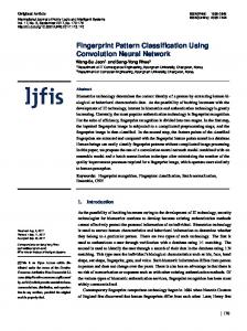
II. EYE BLINK CHARACTERISTICS A. Amplitude The eye related signals will be predominant in the frontal and prefrontal regions of the brain. In the prefrontal lobe, say FP1-F3 or FP2-F4 electrode pairs, a downward peak in the negative region shows an eyes-open event and a positive peak shows an eyes-close event. Also the amplitude of these peaks will be significantly higher compared to the rhythmic brain activity. An eye-blink signal can be detected by its positive and negative peak occurrences.
I. INTRODUCTION An EEG signal is a measurement of currents that flow during synaptic excitations of the dendrites of many pyramidal neurons in the cerebral cortex. When brain cells (neurons) are activated, the synaptic currents are produced within the dendrites. This current generates a magnetic field measurable by electromyogram (EMG) machines and a secondary electrical field over the scalp measurable by EEG systems. In healthy adults, the amplitudes and frequencies of such signals change from one state of a human to another, such as wakefulness and sleep. The characteristics of the waves also change with age. There are five major brain waves distinguished by their different frequency ranges. These frequency bands from low to high frequencies respectively are called alpha (α), theta (θ), beta (β), delta (δ), and gamma (γ). The main artifacts can be divided into patient-related (physiological) and system artifacts. The patient-related or internal artifacts are body movement-related, EMG, ECG (and pulsation), EOG, ballistocardiogram and sweating. The system artifacts are 50/60 Hz power supply interference, impedance fluctuations, cable defects, electrical noise from the electronic components and unbalanced impedances of the electrodes.
Manuscript received March , 2010. Brijil Chambayil, Department of Instrumentation and Control Engineering, National Institute of Technology, Jalandhar, Punjab - 144011, India. (phone: +91-9357710155; e-mail:
[email protected]). Rajesh Singla, Department of Instrumentation and Control Engineering, National Institute of Technology, Jalandhar, Punjab-144011, India. (e-mail:
[email protected]). R. Jha, Department of Instrumentation and Control Engineering, National Institute of Technology, Jalandhar, Punjab-144011, India. (e-mail:
[email protected]).
ISBN: 978-988-17012-9-9 ISSN: 2078-0958 (Print); ISSN: 2078-0966 (Online)
Figure 1.
Eye blink signal
B. Kurtosis The EEG signal is stochastic, and each set of samples is called realizations or sample functions (x(t)). The expectance (µ) is the mean of the realizations and is called first-order central momentum. The second-order central momentum is the variance of the realizations. The square root of the variance is the standard deviation (σ), which measures the spread or dispersion around the mean of the realizations [5]. The kurtosis, also called fourth-order central momentum, characterizes the relative flatness or peakedness of the signal distribution [5], and is defined in (1), which was modified to refer to a non-Gaussian distribution. (1)
The kurtosis coefficient of an event is significantly high when there is an eyes-open, eyes-close or an eye blink. The other spurious signals generated by patient movement, event like switching ON/OFF a plug etc have a small value for kurtosis coefficient. Hence eye events can be detected by kurtosis coefficient. WCE 2010
Proceedings of the World Congress on Engineering 2010 Vol I WCE 2010, June 30 - July 2, 2010, London, U.K.
III. NEURAL NETWORK
V. PREPROCESSING OF DATA FOR NN TRAINING
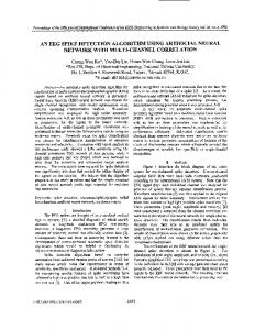
Neural Networks (NN) are simplified models of the biological nervous system and therefore have drawn their motivation from the kind of computing performed by a human brain. An NN, in general, is a highly interconnected network of a large number of processing elements called neurons in an architectur5e inspired by the brain. Neural networks learn by examples. They can therefore be trained with known examples of a problem to ‘acquire’ knowledge about it. Once appropriately trained, the network can be put to effective use of solving ‘unknown’ or ‘untrained’ instances of the problem. Multilayer feed-forward network architecture is made up of multiple layers: an input layer, a number of hidden layers and an output layer. Neurons are the computing elements in each layer. The acceleration or retardation of the input signals is modeled by the weights. The weighted sum of the inputs to each neuron is passed through an activation function to get the output of a neuron. In addition to the inputs there are also biases to each neuron.
The NN will learn the best from the training if the input data and output data fall in the range of [-1, 1].Hence all the data available is preprocessed using ‘PREMNMX’ command in MATLAB to span in the range [-1, 1]. After preprocessing, the entire dataset is divided into two, one for training the neural network and the other for testing the neural network. The training set contains 303 sample windows and the testing set contains 81 sample windows.
Figure 2.
A Multilayer Feed-forward Network
IV. SIGNAL ACQUISITION AND PROCESSING The EEG signal is acquired using RMS EEG 32 Super Spec system. The Ag-AgCl electrodes are placed in the FP1 and F3 region in the 10-20 International electrode system. The leads connected to the Head Box. The Head Box minimizes the noise pickups. The total integration of analog and digital processing in the compact Head Box gives excellent signal to noise ratio too. The Super Spec ensures high-resolution, authentic data acquisition through its software and Head Box. EEG data is acquired from 13 subjects. The acquired data signals are converted into corresponding excel sheets. The signal length is of 15360 samples each. The entire signals taken from the 13 subjects are divided into 512 sample windows. Therefore, in total there are 392 sample windows. The Kurtosis coefficient of each sample window is found out using MATLAB. Also the maximum and minimum amplitudes in each sample window are found out. The eye blink signals are characterized by high value of kurtosis coefficient, normally above the value 3. The data is arranged in excel files as kurtosis of previous samples, kurtosis of present sample, kurtosis of next sample, maximum amplitude and minimum amplitude. These are considered as inputs to the neural network. Also an output set is defined in which the eye blink events are marked as ‘1’ and non-eye blink event as ‘0’.
ISBN: 978-988-17012-9-9 ISSN: 2078-0958 (Print); ISSN: 2078-0966 (Online)
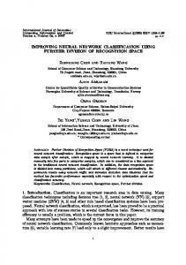
VI. TRAINING, VALIDATION AND TESTING OF NEURAL NETWORK The standard ANN supervised training algorithm for error backpropagation [6] consists of two steps: the forward propagation and the backpropagation. The forward propagation step is achieved by applying a training pattern to the ANN, propagating it through the network and obtaining the continuous output value. This output value is compared to the desired value of the pattern, generating an error value. The error value is backpropagated to adjust the synaptic weights of the neurons, characterizing the backpropagation step. The Cross Validation (CV) procedure [6], applied to the supervised training of neural networks, evaluates the training and the learning of the NN. The CV is executed during the NN training at the end of a training epoch and requires two pattern sets: the training set and the validation set. All training and validation patterns are presented to evaluate the training error and learning error of ANN for that epoch. The errors can be evaluated by the mean square error. If the training algorithm is converging, the training error is falling towards zero. Normally, the learning error falls to the best generalization point, and then continuously increases, which indicates over-training and the loss of generalization. The testing of NN is done by simulating the NN with the testing set and then calculating the error. VII. RESULTS AND DISCUSSION A. Comparison of FFBP and CFBP Network The best performance is obtained in Feed-forward Backpropagation (FFBP) and Cascade-forward Backpropagation (CFBP) networks when compared to other networks. An FFBP network with three layers in 14 : 9 : 1 topology is trained to get an overall regression, R = 0.8499, while in CFBP network with same topology gives a better performance or R = 0.90856. These results were obtained after dozens of training, validation and performance evaluations. TABLE I.
COMPARISON OF FFBP AND CFBP NETWORKS
Regression values[0, 1] Rtrain Rvalidation Rtest Roverall
FFBP 0.96687 0.75527 0.71678 0.84990
CFBP 0.99832 0.80232 0.54784 0.90856
WCE 2010
Proceedings of the World Congress on Engineering 2010 Vol I WCE 2010, June 30 - July 2, 2010, London, U.K.
(a) Regression plot of FFBP training
(b) Regression plot of FFBP validation
(c) Regression plot of FFBP testing
(a) Regression plot of CFBP training
(b) Regression plot of CFBP validation
(c) Regression plot of CFBP testing
(d) Regression plot of FFBP overall
(d) Regression plot of CFBP overall
Figure 3. FFBP regression plots, (a) Regression plot of FFBP training, (b) Regression plot of FFBP validation, (c) Regression plot of FFBP testing, (d) Regression plot of FFBP overall
Figure 4. CFBP regression plots, (a) Regression plot of CFBP training, (b) Regression plot of CFBP validation, (c) Regression plot of CFBP testing, (d) Regression plot of CFBP overall
ISBN: 978-988-17012-9-9 ISSN: 2078-0958 (Print); ISSN: 2078-0966 (Online)
WCE 2010
Proceedings of the World Congress on Engineering 2010 Vol I WCE 2010, June 30 - July 2, 2010, London, U.K.
From the results it is evident that the CFBP network is better compared to the FFBP network and other networks. VIII. CONCLUSION This contribution presented a new application of the neural network classifier to detect the eye blink artifact in the EEG signal. Kurtosis coefficient, maximum amplitude and minimum amplitude in a sample window are successfully used to train the neural network to detect the eye blink signals. The performance of the CFBP network is better compared to the FFBP networks in classifying a signal to an eye blink or not. This classifier can be used to detect the eye blink signals and to further process the signal for BCI applications. REFERENCES [1] [2]
[3] [4]
[5]
[6]
Saeid Sanei and J. A. Chambers, “EEG Signal Processing”, First Edition, ch. 1, p1 – p18, John Wiley and Sons Ltd., 2007. S. Rajasekaran. G. A. Vijayalakshmi Pai, “Neural Networks, Fuzzy Logic and Genetic Algorithms: Synthesis and Applications”, First Edition, ch. 1 – ch. 2, p1 - p33, PHI Learning Private Ltd., 2008. Rajesh Singla, Balraj Gupta, “Brain Initiated Interaction”, Journal of Biomedical Science and Engineering, p170 – p172, 2008. Sovierzoski M.A., Argoud F.I.M., de Azevedo F.M., “Identifying eye blinks in EEG signal analysis“, Proceedings of the 5th International Conference on Information Technology and Application in Biomedicine, p406 - p409, May 2008, China. D. G. Manolakis, V. K. Ingle, S. M. Kogon, “Statistical and Adaptive Signal Processing: Spectral Estimation, Signal Modeling, Adaptive Filtering and Array Processing”, Artech House Publishers, 2005. ch. 3, pp. 75–82. S. Haykin, “Neural Networks: A Comprehensive Foundation”, 1998, Prentice Hall.
ISBN: 978-988-17012-9-9 ISSN: 2078-0958 (Print); ISSN: 2078-0966 (Online)
WCE 2010