This paper examines the capabilities of the Particle Filter (PF) for the tracking ...... F., âParticle Filter Theory and Practice with Positioning Applications,â IEEE ...
AIAA Guidance, Navigation, and Control (GNC) Conference August 19-22, 2013, Boston, MA
AIAA 2013-5243
Comparison of Two Particle Filter Methods For Image Plane Tracking of Multiple Objects Ernest J. Ohlmeyer1 Aero Science Applications LLC, King George, VA 22485 and Downloaded by Domenic Bucco on September 10, 2013 | http://arc.aiaa.org | DOI: 10.2514/6.2013-5243
P. K. Menon2 Optimal Synthesis Inc., Los Altos, CA 94022
Abstract This paper examines the capabilities of the Particle Filter (PF) for the tracking of multiple objects moving on a focal plane array image plane. The study considers the tracking of four objects for which the dynamics are near constant velocity with random perturbations in acceleration. The filtering structure uses four separate PFs rather than a concatenated filter with four sets of target states. There is a data association problem in which each measurement must be assigned to the proper PF. A new association logic based on weighted nearest neighbor strategy is employed to solve this problem. Two new methods are considered for calculating the PF importance weights. The first is based on a weighted distance between the PF position estimate and the perceived location of maximum measurement intensity. The second method employs a likelihood ratio to compute the weights. The first method performed well at a signal-to-noise ratio (SNR) of 15 dB or higher but was unsatisfactory below this. The second method was found to perform well at very low SNR approaching 0 dB. The paper discusses the multiobject tracking scenario, describes the association logic and PF implementations, discusses the analysis details, and shows the performance obtained from the PF.
1 2
Principal Scientist, Associate Fellow AIAA. Chief Scientist and President, Fellow AIAA.
Copyright © 2013 by Ernest J. Ohlmeyer, Aero Science Applications LLC. Published by the American Institute of Aeronautics and Astronautics, Inc., with permission.
I. Introduction
Downloaded by Domenic Bucco on September 10, 2013 | http://arc.aiaa.org | DOI: 10.2514/6.2013-5243
The Particle Filter (PF) is a newly-emerged nonlinear estimation technique based on Bayesian Sequential Monte Carlo Methods which has been found to be very effective in difficult tracking problems where traditional filters such as the Extended Kalman Filter (EKF) break down. Although related ideas have been in the literature since the 1950’s, particle filtering is generally considered to have emerged as a new paradigm in nonlinear estimation in 1993 with the publication of [1]. Since then, PF research has seen explosive growth. The algorithms for implementing a PF have been described extensively in the literature and will not be repeated here. See [1-10] for more detailed and complete descriptions. The basic premise of the PF is to represent the evolving pdf by a fairly large set of random samples, or particles. The particles are stochastic realizations of the state vector. The particle set is propagated in time and updated with new measurements in the familiar predictor-corrector cycle. However, a re-sampling step is usually required during the update [1]. While powerful, the challenge of implementing an estimator such as the PF is to contain the computational complexity while maintaining accuracy so as to permit on-line, real-time processing. The basic version of the PF is simple to implement and often very effective. However, for some difficult tracking problems, a very large set of particles may be required for satisfactory performance. This can occur when most of the prior samples are rejected and just a small subset of the population is re-sampled many times, leading to a phenomenon known as degeneracy. Techniques for dealing with this problem are discussed in the references cited previously. The authors of the present paper have been actively involved in the development of advanced nonlinear estimation techniques for target tracking applications over the past decade [11-16]. The current research is focused on using the PF for tracking of multiple objects (such as a primary target in the presence of one or more secondary objects, sometimes in a background of clutter). These can occur frequently in military scenarios involving target tracking with infrared imaging or radar sensor systems. Further treatment of this advanced PF multi-object tracking topic is given in [17-29].
II. Image Tracking Scenario We consider the tracking of multiple, dynamic targets as they migrate across the image plane. A set of four targets was chosen for analysis and their motions are illustrated in Fig. 1. The targets are initially located in the corners of the array, converge toward the center with some crossing each other, and then continue on to the array edges. Also shown are the target velocity and heading angle histories. The array dimensions are 256 x 256 pixels and the maximum scenario time is 10 s. The targets experience random normal and longitudinal accelerations which introduce perturbations to the baseline constant velocity, straight line motion. The
Copyright © 2013 by Ernest J. Ohlmeyer, Aero Science Applications LLC. Published by the American Institute of Aeronautics and Astronautics, Inc., with permission.
Assumed Target Motion (4 Targets) locations of the four targets at selected time points are shown superimposed on the array’s background noise for a 15 dB SNR in Fig. 2. TARGET POSITIONS
TARGET TOTAL VELOCITIES
250
TARGET HEADING ANGLES
25
150
24 100 23
TGT 1 TGT 2 TGT 3 TGT 4
50 VT (PIXELS/S)
150
100
22
GAMMA (DEG)
Downloaded by Domenic Bucco on September 10, 2013 | http://arc.aiaa.org | DOI: 10.2514/6.2013-5243
Y (PIXELS)
200
21 20
0
-50
TGT 1 TGT 2 TGT 3 TGT 4
19 50
-100 18
0
0
50
100 150 X (PIXELS)
200
250
17
0
5 T (SEC)
10
-150
0
5 T (SEC)
10
Fig. 1. Assumed Target Motions in Image Plane
Fig. 2. Target Locations in Measurement Plane at Selected Times (SNR = 15 dB) The true target dynamics are shown in Fig. 3 and consist of a perturbed constant acceleration model. States are x and y position, total velocity (V) and heading angle (), and longitudinal (aL) and normal (aN) accelerations with respect to the velocity vector. The jerk, or rate of change of acceleration, is modeled as random Gaussian noise with standard deviations of L = 0.5 pixels/s2
Copyright © 2013 by Ernest J. Ohlmeyer, Aero Science Applications LLC. Published by the American Institute of Aeronautics and Astronautics, Inc., with permission.
x V cos( ) 0 0 y V sin( ) 0 0 V aL 0 0 wL a / V 0 0 N wN and N = 1.0 pixels/s2 at a time step of t = 0.1 s. The tracking is performed by four separate a L 0 1 0 particle filters where the model used in each filter is given in Fig. 4. In this case, each filter has four states consisting of x, y positions and velocities 0 coordinates. 0 1This nearly a Nin Cartesian constant velocity model is driven by random x, y accelerations (w) with a standard deviation of w = 0.5 pixels/s2 at t = 0.1 s.
X f ( X ) B w(t )
TargetConstant Truth Model Acceleration Model in Velocity-Fixed Axes
Simplified
(k 1) ( V (k 1) V ( aL (k 1) a a N (k 1) a
Random accelerations:
Downloaded by Domenic Bucco on September 10, 2013 | http://arc.aiaa.org | DOI: 10.2514/6.2013-5243
X [x
y
V
wL , wN N (
a N ]T
aL
x V cos( ) 0 y V sin( ) 0 V a L 0 a N / V 0 a L 1 0 0 0 a N
y
0 0 0 wL 0 wN 0 1
1
Longitudinal aN v (k 1)pixel V Assume w(t) is piecewise L constant over T tk 1x tk accel
a
) TV= a L 0v.y5(k 1at
Normal accel
Integration aSimplified V VelocityAlgorithm N (k 1) (k ) Heading [a N (k ) /angle V (k )]T V (k 1) V (k ) a L (k )T a L (k 1) a L (k ) wL (k ) x a N (k 1) a N (k ) wN (k )
X f ( X ) B w(t )
a x (k 1) a
a y (k 1) a
x(k 1) x(k
y(k 1) y(
Random accelerations: aL , 2aN
w , w N (0, w ) Particle Filter ModelL N 1 a N Model 3. Target Truth v (k 1)pixel/s V (k2 1) cos[ (k 1)] aFig. L( For each of 4 separate xfilters) ) TV=(k0.1 1s) sin[ (k 1)] a L 0v.y5(k 1at
Longitudinal accel
y
a x (k 1) a L (k 1) cos[ (k 1)] a N (k 1) sin[ (k 1)]
Normal accel
aN
V
Velocity
X x yangle vx Heading
vy
r T
T
a y (k T 1) a L (k 1) sin[ (k 1)] a N (k 1) cos[ (k 1)]
v
T
x(k 1) x(k ) v x (k 1)T 12 a x (k 1)T 2 y (k 1) y (k ) v y (k 1)T 12 a y (k 1)T 2
r k 1 I 2 v 0 k 1 2
Tx I 2 r k 12 T 2 I 2 w k I 2 v k T I 2
X k 1 X k w k
w 0.5
pixel/s2 at T = 0.1 s
Fig. 4. Filter Model
The measurement set Z consists of a 256 x 256 set of measured intensities in the image plane. The distortion of the measured intensities is modeled by a Gaussian point spread function with blur parameter = 2 pixels and nominal amplitude A = 1. In the analysis, the signal-to-noise
Copyright © 2013 by Ernest J. Ohlmeyer, Aero Science Applications LLC. Published by the American Institute of Aeronautics and Astronautics, Inc., with permission.
ratio (SNR, dB) was parametrically varied and the corresponding image noise standard deviation (Z) was calculated using the relation: Z = A/10SNR/20.
Downloaded by Domenic Bucco on September 10, 2013 | http://arc.aiaa.org | DOI: 10.2514/6.2013-5243
III. Data Association Problem In the multi-target tracking scenario, the possibility of incorrect association between the various filters and measurements must be considered. The current analysis employed a data association logic based on the nearest neighbor method. For each of the four filters, the distances from each of the N prior particle positions to each of the four measurement peak intensity locations (x*, y*) are computed. Using the last prior weight set from each filter, the weighted mean of the distances from the i-th filter to the j-th peak is calculated over the N particles. Then, each filter associates with itself the measurement having the smallest mean weighted distance. This technique for data association was used in both multi-target tracking methods described in Sections IV and V below. Details of the association algorithm are as follows: Let the prior particle sets and their associated normalized weights for the n-th particle and the i-th filter be denoted by:
{xˆ in , yˆ in , win }in11::4N The coordinates of the j-th peak measured intensity on the image plane are written as:
{x*j , y*j}j1:4 The distance from the n-th particle of the i-th filter to the j-th peak is given by:
rin, j ( xˆ in x*j ) 2 ( yˆ in y*j )2 The weighted mean distance from the i-th filter to the j-th measurement peak is computed as: N
R w in rin, j j i
n 1
Then, the i-th filter uses the measurement j*, where j* is the index corresponding to:
R ij* min{R ij} j
Copyright © 2013 by Ernest J. Ohlmeyer, Aero Science Applications LLC. Published by the American Institute of Aeronautics and Astronautics, Inc., with permission.
IV. PF Tracking Method #1 Use of the PF for multi-target tracking was implemented using two methods. In Method #1, the importance weights were generated as shown in Fig. 5. The location (x*, y*) of the maximum measured intensity for each measurement set is first determined. Then, the distances (rn) between the estimated position coordinates of the n-th prior particle (xn, yn) and the peak intensity locations (x*, y*) are calculated. The weights are computed using the formula at the bottom of Fig. 5, which is an exponential function of (rn/r1)2 where the design parameter r1 was chosen as 1.0 pixel.
Downloaded by Domenic Bucco on September 10, 2013 | http://arc.aiaa.org | DOI: 10.2514/6.2013-5243
Generation of Importance Weights from Image Data
Coordinates (x*,y*) at peak intensity Zmax
Point spread function for measured intensity Z(x,y)
Coordinates (xn, yn) of n-th prior particle rn
n-th importance weight
r1 is design parameter
Wn exp{ 1 2 [( x * xn ) 2 ( y * yn ) 2 ] / r1 } exp{ 1 2 rn2 / r1 } 2
2
Fig. 5. Generation of Importance Weights from Image Data (Method #1)
Tracking results using Method #1 are shown for SNR = 15 dB. For this case the PF used 10,000 particles. Fig. 6 displays the true target positions and the estimated particle clouds at selected time points. The position estimation errors and 2- bounds for each target are shown in Fig. 7. The results indicate accurate and consistent tracking with Method #1 at this SNR. The performance of the data association logic is illustrated in Fig. 8. The weighted distances are shown from each filter (X1-X4) to each measurement peak (Z1-Z4). It is seen that for this SNR each filter is associated with the correct measurement, as identified by the smallest distance.
Copyright © 2013 by Ernest J. Ohlmeyer, Aero Science Applications LLC. Published by the American Institute of Aeronautics and Astronautics, Inc., with permission.
Position Tracking Errors and 2- Bounds POS ERRORS - TGT 1
POS ERRORS - TGT 2
0
5 T (SEC)
-1 -2
10
0
5 T (SEC)
0 -1
0
5 T (SEC)
10
1 0 -1 -2
0 -1
0
5 T (SEC)
0
5 T (SEC)
10
0 -1
0
5 T (SEC)
10
0
5 T (SEC)
10
2
1 0 -1 -2
1
-2
10
2 Y ERROR (PIXELS)
1
1
-2
10
2 Y ERROR (PIXELS)
2
-2
0
X ERROR (PIXELS)
-1
1
2
Y ERROR (PIXELS)
0
POS ERRORS - TGT 4
2 X ERROR (PIXELS)
1
-2
POS ERRORS - TGT 3
2 X ERROR (PIXELS)
X ERROR (PIXELS)
2
Y ERROR (PIXELS)
Downloaded by Domenic Bucco on September 10, 2013 | http://arc.aiaa.org | DOI: 10.2514/6.2013-5243
Fig. 6. Method #1 Tracking Results, SNR = 15 dB
0
5 T (SEC)
10
1 0 -1 -2
Fig. 7. Method #1 Position Estimation Errors and 2- Bounds, SNR = 15 dB
Copyright © 2013 by Ernest J. Ohlmeyer, Aero Science Applications LLC. Published by the American Institute of Aeronautics and Astronautics, Inc., with permission.
Weighted Distance, X1 TO Z1-Z4
Weighted Distance, X2 TO Z1-Z4 300
Z1 Z2 Z3 Z4
200
D (PIXELS)
D (PIXELS)
300
100
0
5 10 T (SEC) Weighted Distance, X3 TO Z1-Z4
0
5 10 T (SEC) Weighted Distance, X4 TO Z1-Z4
300
D (PIXELS)
D (PIXELS)
Downloaded by Domenic Bucco on September 10, 2013 | http://arc.aiaa.org | DOI: 10.2514/6.2013-5243
100
0
0
300
200
100
0
200
0
5 T (SEC)
10
200
100
0
0
5 T (SEC)
10
Fig. 8. Method #1 Mean Weighted Distances vs Time, SNR = 15 dB Further analysis of Method #1 indicated that while excellent tracking performance was obtained at fairly high SNR ( 15 dB), the filter performance rapidly deteriorated below this point with eventual collapse of the filter solution. This seems somewhat intuitive since Method #1 relies on being able to distinguish the peak intensity location on the array in the presence of noise. As SNR decreases, the ability to discern this peak becomes increasingly difficult, as evidenced by the problem of visually picking the target out of low SNR images. As a result of this limitation, an alternate Method #2 was examined.
V. PF Tracking Method #2 This method borrows ideas from the track-before-detect literature [3, 4 (chapter 11)] but extends them by considering multiple targets and by employing a data association logic based on nearest neighbor using mean weighted distance (see Section III). Method #2 uses a technique in which the weights are computed from a likelihood ratio, which will be defined below. A number of assumptions have been employed in the present analysis and are listed below:
The targets have been previously detected and always exist thereafter. (i.e., the detection problem is not explicitly addressed but could be considered in an expanded analysis)
The number of targets is constant and known (in this case, four).
There are four PFs, each assigned to one target.
The filters are initialized with reasonably small errors: 3 pixels and 0.5 pixels/s maximum errors, uniformly distributed. (The sensitivity to initialization errors will be examined later.)
Copyright © 2013 by Ernest J. Ohlmeyer, Aero Science Applications LLC. Published by the American Institute of Aeronautics and Astronautics, Inc., with permission.
The measurement model for the n-th particle in cell (i, j) is a Gaussian point spread function with amplitude A and blur parameter :
(i xˆ n ) 2 ( j yˆ n ) 2 z ( i, j) h ( i, j) ( xˆ n , yˆ n ) A exp 2 2 In the analysis, the assumed filter values of A and were chosen to be different from the true values.
Downloaded by Domenic Bucco on September 10, 2013 | http://arc.aiaa.org | DOI: 10.2514/6.2013-5243
The likelihoods in cell (i, j) for signal plus noise and for noise alone are given by:
pS( i, jN) p(z ( i, j) | xˆ n , yˆ n ) (z ( i, j) ; h ( i, j) , 2Z ) p(Ni, j) p(z ( i, j) ) (z ( i, j) ;0, 2Z ) where
(z ( i, j) ; h( i, j) , 2Z ) exp (z ( i, j) h( i, j) )2 / 22Z
Division of these gives the likelihood ratio:
( i , j)
h ( i , j ) ( h ( i , j ) 2z ( i , j ) ) pS( i, jN) exp p(Ni, j) 22Z
Method #2 uses the likelihood ratio to calculate the unnormalized weights. Assuming the measurement noise is independent from pixel to pixel, these are given by:
~ n ( i , j) w iC jC
where C is a region of D pixels about the (x, y) position estimate of the n-th prior particle. In the current analysis D = 10 pixels was used. A summary of the parameters used in the evaluation of Method #2 is provided in Table 1.
Copyright © 2013 by Ernest J. Ohlmeyer, Aero Science Applications LLC. Published by the American Institute of Aeronautics and Astronautics, Inc., with permission.
Downloaded by Domenic Bucco on September 10, 2013 | http://arc.aiaa.org | DOI: 10.2514/6.2013-5243
Parameter
Assumed Value
Number of particles, N
10,000
Time step, T (for both propagate & update)
0.1 s
Target 1- normal accel, AN
1.0 pixel/s2
Target 1- longitudinal accel, AL
0.5 pixel/s2
Filter process noise 1- x, y accel, W
0.5 pixel/s2
Initial conditions (x, y)max (uniform)
3.0 pixels
Initial conditions (vx, vy)max (uniform)
0.5 pixels/s
Signal-to-noise ratio, SNR
2, 6, 15 dB
True amplitude, ASIGNAL
1.0
Estimated amplitude
0.8 * ASIGNAL
True 1- image noise, Z
ASIGNAL / (10SNR/20)
Estimated 1- image noise
1.5 * Z
True blur parameter,
2.0 pixels
Estimated blur parameter
1.5 *
Focal plane array dimensions
256 x 256 pixels
Box ( D) about estimated (x, y) used in weight calc
10 pixels
Table 1. Assumed Parameters for Method #2
Results for Method #2 are now provided as a function of SNR. The tracking performance of Method #2 at SNR = 15 dB was found similar to Method #1 but was somewhat more accurate. Fig. 9 shows the true and estimated target tracks and Fig. 10 shows the position estimation errors and their 2- bounds. The tracking errors are seen to be very small, a small fraction of a pixel. The data association algorithm is assessed in Fig. 11, which displays flags for each filter that indicate whether the filter-target association was correct (value = 1) or incorrect (value = 0). Next to the filter number is shown the probability of correct associations (PCA) computed over the tracking interval. For this SNR, the PCA is very high, ranging from 98-100 percent.
Copyright © 2013 by Ernest J. Ohlmeyer, Aero Science Applications LLC. Published by the American Institute of Aeronautics and Astronautics, Inc., with permission.
Position Tracking Errors & 2- Bounds, SNR = 15 dB
POS ERRORS - TGT 1
POS ERRORS - TGT 2
0
5 T (SEC)
-1 -2
10
0
5 T (SEC)
0 -1
0
5 T (SEC)
10
1 0 -1 -2
0 -1
0
5 T (SEC)
0
5 T (SEC)
10
0 -1
0
5 T (SEC)
10
0
5 T (SEC)
10
2
1 0 -1 -2
1
-2
10
2 Y ERROR (PIXELS)
1
1
-2
10
2 Y ERROR (PIXELS)
2
-2
0
X ERROR (PIXELS)
-1
1
2
Y ERROR (PIXELS)
0
POS ERRORS - TGT 4
2 X ERROR (PIXELS)
1
-2
POS ERRORS - TGT 3
2 X ERROR (PIXELS)
X ERROR (PIXELS)
2
Y ERROR (PIXELS)
Downloaded by Domenic Bucco on September 10, 2013 | http://arc.aiaa.org | DOI: 10.2514/6.2013-5243
Fig. 9. Method #2 Tracking Results, SNR = 15 dB
0
5 T (SEC)
10
1 0 -1 -2
Fig. 10. Method #2 Position Estimation Errors and 2- Bounds, SNR = 15 dB
Copyright © 2013 by Ernest J. Ohlmeyer, Aero Science Applications LLC. Published by the American Institute of Aeronautics and Astronautics, Inc., with permission.
1
0.5
0 50 UPDATE NUMBER
1
0.5
0 0
50 UPDATE NUMBER
1
0.5
0
100
FILTER 4 PCA = 100.00
FILTER 3 PCA = 99.01
0
0
50 UPDATE NUMBER
100
0
50 UPDATE NUMBER
100
1
0.5
0
100
Fig. 11. Method #2 Correct Association Indicators for Each Filter, SNR = 15 dB To further verify algorithm consistency, Fig. 12 provides plots of the measurement residuals and 2- bounds. Although there is actually a residual for each cell in the array, and for each of the N particles, the residuals here were computed as the differences between the measured and modeled intensities in the cell nearest to each prior particle location. Then a weighted mean and variance calculation was performed over the N residual values. The residual means and standard deviations so derived are plotted in Fig. 12 and indicate consistent behavior. RESIDUALS - FILTER 2 2
1
1
RESIDUAL
2
0 -1 -2
0
5 T (SEC) RESIDUALS - FILTER 3
0 -1 -2
10
2
2
1
1
RESIDUAL
RESIDUAL
RESIDUALS - FILTER 1
RESIDUAL
Downloaded by Domenic Bucco on September 10, 2013 | http://arc.aiaa.org | DOI: 10.2514/6.2013-5243
SNR = 15 DB
FILTER 2 PCA = 98.02
FILTER 1 PCA = 100.00
CORRECT ASSOCIATION INDICATOR
0 -1 -2
0
5 T (SEC)
10
0
5 T (SEC) RESIDUALS - FILTER 4
10
0
5 T (SEC)
10
0 -1 -2
Fig. 12. Method #2 Measurement Residuals & 2- Bounds for Each Filter
Copyright © 2013 by Ernest J. Ohlmeyer, Aero Science Applications LLC. Published by the American Institute of Aeronautics and Astronautics, Inc., with permission.
Fig. 13. Method #2 Tracking Results, SNR = 6 dB Position Tracking Errors & 2- Bounds, SNR = 6 dB POS ERRORS - TGT 1
POS ERRORS - TGT 2
0
5 T (SEC)
0
5 T (SEC)
0 -2
0
5 T (SEC)
10
2 0 -2 -4
0 -2
0
5 T (SEC)
0
5 T (SEC)
10
0 -2
0
5 T (SEC)
10
0
5 T (SEC)
10
4
2 0 -2 -4
2
-4
10
4 Y ERROR (PIXELS)
2
2
-4
10
4 Y ERROR (PIXELS)
Y ERROR (PIXELS)
-2 -4
10
4
-4
0
X ERROR (PIXELS)
-2
2
4
Y ERROR (PIXELS)
0
POS ERRORS - TGT 4
4 X ERROR (PIXELS)
2
-4
POS ERRORS - TGT 3
4 X ERROR (PIXELS)
4 X ERROR (PIXELS)
Downloaded by Domenic Bucco on September 10, 2013 | http://arc.aiaa.org | DOI: 10.2514/6.2013-5243
In sharp contrast to Method #1, Method #2 was able to maintain accurate tracking at very low SNR. Results for SNR = 6 dB are shown in Figs. 13 through 15. The true and estimated target tracks are displayed in Fig. 13. The position estimation errors in Fig. 14 are larger than those at 15 dB, but, except for a few transient excursions, tracking is being performed to within 1-2 pixels most of the time and the tracking errors are generally contained within their statistical bounds. The data association indicator history in Fig. 15 shows that at SNR = 6 dB, the PCA is between 26-40 percent, with an average of 30.7.
0
5 T (SEC)
10
2 0 -2 -4
Fig. 14. Method #2 Position Estimation Errors and 2- Bounds, SNR = 6 dB
Copyright © 2013 by Ernest J. Ohlmeyer, Aero Science Applications LLC. Published by the American Institute of Aeronautics and Astronautics, Inc., with permission.
1
0.5
0 50 UPDATE NUMBER
1
0.5
0 0
50 UPDATE NUMBER
1
0.5
0
100
FILTER 4 PCA = 39.60
FILTER 3 PCA = 26.73
0
Downloaded by Domenic Bucco on September 10, 2013 | http://arc.aiaa.org | DOI: 10.2514/6.2013-5243
SNR = 6 DB
FILTER 2 PCA = 27.72
FILTER 1 PCA = 28.71
CORRECT ASSOCIATION INDICATOR
100
0
50 UPDATE NUMBER
100
0
50 UPDATE NUMBER
100
1
0.5
0
Fig. 15. Method #2 Correct Association Indicators for Each Filter, SNR = 6 dB Method #2 was also found to give very satisfactory performance at SNR = 2 dB. These results are shown in Figs. 16 through 18. Correct data associations were made between 23-34 percent of the time with an average of 27.5. The PCA (averaged over the tracking interval and over four filters) was computed for a range of SNR values and these results are shown in Fig. 19. For Method #2, correct associations are made about 27 percent of the time at SNR = 0 dB, 50 percent of the time at SNR = 9 db, and 100 percent of the time for SNR 15 dB. In contrast, Method #1 is seen to have much poorer association performance.
Fig. 16. Method #2 Tracking Results, SNR = 2 dB
Copyright © 2013 by Ernest J. Ohlmeyer, Aero Science Applications LLC. Published by the American Institute of Aeronautics and Astronautics, Inc., with permission.
Position Tracking Errors & 2- Bounds, SNR = 2 dB
POS ERRORS - TGT 1
POS ERRORS - TGT 2
0
5 T (SEC)
0
5 T (SEC)
0 -2
0
5 T (SEC)
10
2 0 -2 -4
0 -2
0
5 T (SEC)
0
5 T (SEC)
0 -2
0
5 T (SEC)
10
0
5 T (SEC)
10
4
2 0 -2 -4
10
2
-4
10
4 Y ERROR (PIXELS)
2
2
-4
10
4 Y ERROR (PIXELS)
Y ERROR (PIXELS)
0
5 T (SEC)
10
2 0 -2 -4
Fig. 17. Method #2 Position Estimation Errors and 2- Bounds, SNR = 2 dB
SNR = 2 DB
FILTER 2 PCA = 26.73
FILTER 1 PCA = 25.74
CORRECT ASSOCIATION INDICATOR 1
0.5
0 50 UPDATE NUMBER
1
0.5
0 0
50 UPDATE NUMBER
1
0.5
0
100
FILTER 4 PCA = 33.66
0
FILTER 3 PCA = 23.76
Downloaded by Domenic Bucco on September 10, 2013 | http://arc.aiaa.org | DOI: 10.2514/6.2013-5243
-2 -4
10
4
-4
0
X ERROR (PIXELS)
-2
2
4
Y ERROR (PIXELS)
0
POS ERRORS - TGT 4
4 X ERROR (PIXELS)
2
-4
POS ERRORS - TGT 3
4 X ERROR (PIXELS)
X ERROR (PIXELS)
4
100
0
50 UPDATE NUMBER
100
0
50 UPDATE NUMBER
100
1
0.5
0
Fig. 18. Method #2 Correct Association Indicators for Each Filter, SNR = 2 dB
Copyright © 2013 by Ernest J. Ohlmeyer, Aero Science Applications LLC. Published by the American Institute of Aeronautics and Astronautics, Inc., with permission.
PROBABILITY OF CORRECT ASSOCIATION VS SNR 110 100 Method 2 Method 1
90
PCA (PERCENT)
Downloaded by Domenic Bucco on September 10, 2013 | http://arc.aiaa.org | DOI: 10.2514/6.2013-5243
80 70 60 50 40 30 20 10 0
0
5
10 SNR (DB)
15
20
Fig. 19. Probability of Correct Association vs SNR
The sensitivity to initial condition uncertainty was evaluated using a slightly different scenario, as shown in Fig. 20. It was assumed that the particles were initialized according to a uniform distribution over a region Xmax pixels about the true target x, y positions and over Vmax pixels/s about the true x, y velocities. The values of Xmax and Vmax were made increasingly larger until the accuracy of the target tracking started to break down. As seen in Fig. 20 for SNR = 2 dB, acceptable tracking with Method #2 is maintained for initial uncertainties up to about Xmax = 7-10 pixels and Vmax = 1.5-2.0 pixels/s.
Copyright © 2013 by Ernest J. Ohlmeyer, Aero Science Applications LLC. Published by the American Institute of Aeronautics and Astronautics, Inc., with permission.
Initial Particle Distribution is Uniform ─> True Position Xmax, True Velocity Vmax
Downloaded by Domenic Bucco on September 10, 2013 | http://arc.aiaa.org | DOI: 10.2514/6.2013-5243
Xmax = 5, Vmax = 1
Xmax = 7, Vmax = 1.5
Xmax = 10, Vmax = 2
Xmax = 20, Vmax = 5
Fig. 20. Tracking Sensitivity to Initial Condition Uncertainty, SNR = 2 dB
VI. Summary and Conclusions This paper investigated two methods for performing multi-target tracking with a PF. The first method computed importance weights based on an exponential function of the distance from the PF estimated position to the location of the peak measured intensity. Method #1 was found to perform well at SNR 15 dB, but rapidly deteriorated below that. Since good performance at low SNR was desired, a second method was investigated. Method #2 utilized track-before-detect techniques and computed the importance weights based on a likelihood ratio function. This method was shown to give excellent tracking performance down to low SNR approaching 0 dB. A new data association algorithm was proposed based on a weighted nearest neighbor strategy and was evaluated in the study. The probability of correct association was determined as a function of SNR. The influence of initial condition uncertainty was also evaluated.
Copyright © 2013 by Ernest J. Ohlmeyer, Aero Science Applications LLC. Published by the American Institute of Aeronautics and Astronautics, Inc., with permission.
VII.
Acknowledgement
This research was supported under MDA Contract No. HQ0006-10-C-7267, with Dr. Demetrios Serakos of the Naval Surface Warfare Center, Dahlgren Division as the technical monitor. We thank Dr. Serakos for his interest and suggestions on several aspects of our work.
References
Downloaded by Domenic Bucco on September 10, 2013 | http://arc.aiaa.org | DOI: 10.2514/6.2013-5243
1. Gordon, N.J., Salmond, D.J. and Smith, A.F.M., “Novel Approach to Nonlinear/Non-Gaussian Bayesian State Estimation,” IEE-Proceedings-F, Vol. 140, No.2, pp. 107-113, 1993. 2. Kitagawa, G., “Monte Carlo Filter and Smoother for Non-Gaussian Nonlinear State Space Models,” J. Comput. Graph. Statist., 5, 1-25, 1996. 3. Salmond, D. J. and Birch, H., “A Particle Filter for Track-Before-Detect,” American Control Conference, Arlington, VA, 2001. 4. Ristic, Branko, Arulampalam, Sanjeev, and Gordon, Neil, Beyond the Kalman Filter: Particle Filters for Tracking Applications, Artech House, Norwood, MA, 2004. 5. Salmond, D. J., “An Introduction to Particle Filters for Tracking and Guidance,” Chapter 12 in: Advances in Missile Guidance, Control and Estimation, S. N. Balakrishnan, et al. Ed., CRC Press, 2013. 6. Arulampalam, M. S., Maskell, S., Gordon, N., and Clapp, T., “A Tutorial on Particle Filters for Online Nonlinear/Non-Gaussian Bayesian Tracking,” IEEE Trans. Signal Processing, Vol. 50, No. 2, February 2002, pp.174-188. 7. Gustafsson, F., “Particle Filter Theory and Practice with Positioning Applications,” IEEE Aerospace and Electronic Systems Magazine, Vol. 25, No. 7, July 2010. 8. Doucet, A., De Freitas, N., and Gordon, N.J. (editors), Sequential Monte Carlo Methods in Practice, New York, Springer-Verlag, 2001. 9. Simon. Dan, Optimal State Estimation, Wiley Interscience, New York, 2006. 10. Thrun, S., Burgard, W. and Fox, D., Probabilistic Robotics, MIT Press, Cambridge, MA, 2005. 11. Kim, J., Vaddi, S. S., Menon, P. K., and Ohlmeyer, E. J., "Comparison Between Nonlinear Filtering Techniques for Spiraling Ballistic Missile State Estimation," IEEE Transactions on Aerospace and Electronic Systems, Vol. 48, No. 1, January 2012. 12. Kim, J., Tandale, M. D., Menon, P. K., and Ohlmeyer, E. J., "A Particle Filter for Tracking a Ballistic Target Under Glint Noise," Journal of Guidance, Control, and Dynamics, Vol. 33, No. 6, NovemberDecember 2010, pp. 1918-1921. 13. Ohlmeyer, E. J., Menon, P. K. and Kim, J., “Tracking of Spiraling Reentry Vehicles with Varying Frequency Using the Unscented Kalman Filter,” AIAA Guidance, Navigation, and Control Conference, Toronto, Canada, August 2-5, 2010.
Copyright © 2013 by Ernest J. Ohlmeyer, Aero Science Applications LLC. Published by the American Institute of Aeronautics and Astronautics, Inc., with permission.
14. Kim, J., Menon, P. K., and Ohlmeyer, E. J., “Motion Models for use with Maneuvering Ballistic Missile Tracking Estimators,” AIAA Guidance, Navigation, and Control Conference, Toronto, Canada, August 2-5, 2010. 15. Vaddi, S. S., Menon, P. K., and Ohlmeyer, E. J., “Target State Estimation for Integrated GuidanceControl of Missiles,” AIAA Guidance, Navigation, and Control Conference, Hilton Head, SC, August 20-23, 2007. 16. Ohlmeyer, E. J. and Menon, P. K., “Applications of the Particle Filter for Multi-Object Tracking and Classification,” American Control Conference, Washington, DC, June 17-19, 2013.
Downloaded by Domenic Bucco on September 10, 2013 | http://arc.aiaa.org | DOI: 10.2514/6.2013-5243
17. Bar-Shalom, Y. and Fortmann, T. E., Tracking and Data Association, Academic Press, New York, 1988. 18. Blackman, S. and Popoli, R., Design and Analysis of Modern Tracking Systems, Artech House, Norwood, MA, 1999. 19. Stone, L. D., Barlow, C. A. and Corwin, T. L., Bayesian Multiple Target Tracking, Artech House, Norwood, MA, 1999. 20. Bar-Shalom, Y. and Li, X., Multitarget-Multisensor Tracking: Principles and Techniques, YBS Publishing, Storrs, CT, 1995. 21. Ng, W., Li, J., Godsill, S. and Vermaak, J., “A Review of Recent Results in Multiple Target Tracking,” Proc. 4th International Symposium on Image and Signal Processing and Analysis, 2005. 22. Pulford, G. W., “Taxonomy of Multiple Target Tracking Methods,” IEE Proc. Radar, Sonar and Navigation, Vol. 152, Issue 5, Oct. 2005. 23. Vermaak, J., Godsill, S. and Perez, P., “Monte Carlo Filtering for Multi-Target Tracking and Data Association,” IEEE Transactions on Aerospace and Electronic Systems, Vol. 41, No. 1, January 2005. 24. Morelande, M., Kreucher, C. and Kastella, K., “A Bayesian Approach to Multiple Target Detection and Tracking,” IEEE Transactions on Signal Processing, Vol. 55, No. 5, May 2007. 25. Musicki, D. and La Scala, B., “Multi-Target Tracking in Clutter without Measurement Association,” IEEE Transactions on Aerospace and Electronic Systems, Vol. 44, No. 3, July 2008. 26. Kreucher, C., Kastella, K. and Hero, A., “Multitatget Tracking using the Joint Multitarget Probability Density,” IEEE Transactions on Aerospace and Electronic Systems, Vol. 41, No. 4, October 2005. 27. Salmond, D. J., Fisher, D. and Gordon, N. J., “Tracking and Identification for Closely Spaced Objects in Clutter,” Proceedings of the European Control Conference, Brussels, 1997. 28. Salmond, D. J., Fisher, D. and Gordon, N. J., “Tracking in the Presence of Intermittent Spurious Objects and Clutter,” in Signal and Data Processing of Small Targets 1998, O. E. Drummond, Ed., Proceedings of the SPIE, Vol. 3373, pp.460-474, 1998. 29. Salmond, D. J. and Gordon, N. J., “Group Tracking with Limited Sensor Resolution and Finite Field of View,” in Signal and Data Processing of Small Targets 2000, O. E. Drummond, Ed., Proceedings of the SPIE, Vol. 4048, pp. 532-540, 2000.
Copyright © 2013 by Ernest J. Ohlmeyer, Aero Science Applications LLC. Published by the American Institute of Aeronautics and Astronautics, Inc., with permission.