1732
IEEE Transactions on Ultrasonics, Ferroelectrics, and Frequency Control ,
vol. 60, no. 8,
August
2013
Comparison of Ultrasonic Array Imaging Algorithms for Nondestructive Evaluation Jie Zhang, Bruce W. Drinkwater, and Paul D. Wilcox Abstract—Ultrasonic array imaging algorithms have been widely used and developed in nondestructive evaluation in the last 10 years. In this paper, three imaging algorithms [total focusing method (TFM), phase-coherent imaging (PCI), and spatial compounding imaging (SCI)] are compared through both simulation and experimental measurements. In the simulation, array data sets were generated using a hybrid forward model containing a single defect among a multitude of randomly distributed point scatterers to represent backscatter from material microstructure. The number of point scatterers per unit area and their scattering amplitude were optimized to reduce computation cost. The SNR of the final images and their resolution were used to indicate the quality of the different imaging algorithms. The images of different types of defects (point reflectors and planar cracks) were used to investigate the robustness of the imaging algorithms. It is shown that PCI can yield higher image resolution and higher SNR for defects in material with weak backscatter than TFM, but that the images of cracks are distorted. Overall, TFM is the most robust algorithm across a range of different types of defects. It is also shown that the detection limit of all three imaging algorithms is almost equal for weakly scattering defects.
I. Introduction
D
etecting and characterizing defects using ultrasonic arrays is an important area in nondestructive evaluation (NDE) [1]. By firing the array elements in predefined sequences (often termed a delay law), one array probe can steer and focus the physical wavefront to many locations in a test structure [2]. This allows real-time images of the test structure to be generated, for example, planar and focused B-scans [3], [4]. Alternatively, the time-domain signals from every pair of transmitter–receiver elements (termed the full matrix of array data) can be captured and post-processed to form an image. The post-processing approach means that a given focused beam is never physically present in the test structure but instead its effect is synthesized by an imaging algorithm applied to the full matrix of array data. A high-resolution image can be reconstructed by synthetically focusing at every image pixel through imaging algorithms such as inverse wave-field extrapolation (IWEX) [5], total focusing method (TFM), [6] and wavenumber algorithm [7]. Although these methods are conceptually different, they can all be expressed in the form of a linear superposition of phase-delayed transmitManuscript received January 4, 2013; accepted May 14, 2013. This work was supported through the core research program within the UK Research Centre in NDE (RCNDE) funded by the Engineering and Physical Sciences Research Council (EPSRC) (grant number EP/F017332/1). The authors are with the Department of Mechanical Engineering, University of Bristol, Bristol, UK (e-mail:
[email protected]). DOI http://dx.doi.org/10.1109/TUFFC.2013.2754 0885–3010/$25.00
ter–receiver signals in the frequency domain with different amplitude coefficients for each image point [8]. The phase delay is the same in all cases and is associated with wave propagation from the transmitter to the image point and back to the receiver. If the point is associated with a scatterer, the coherent summation results in a high intensity. Nonlinear denoising algorithms, such as spatial compounding imaging (SCI) [9]–[12] and phase-coherence imaging (PCI) [13]–[16], can be further used to reduce uncorrelated material noise and improve the image quality in both medical and engineering applications. The procedures use the statistical characteristics of the intensity contribution from specific transmitter–receiver pairs or sub-arrays. In spatial compounding techniques, a pixel located within a test structure is observed from various sub-arrays [11] at different inspection angles. The final image is the superposition of chosen sub-array images. In phase coherence imaging techniques, the final image is a linear ultrasound scan image multiplied by a coherence weighting function [13]. The coherence weighting function is associated with the statistical characteristics of the phase information from a point reflector or material grain scatterer in a structure. Through this weighting function, the intensities of the image pixels associated with material grain backscattering are attenuated. The purpose of this paper is to propose a methodology to qualitatively and quantitatively assess the suitability of imaging algorithms for NDE, especially for inspecting material with strong backscatter. Compared with other linear imaging algorithms [3], [4], the TFM, wavenumber, and back propagation imaging algorithms have higher resolution and SNR [8]. However, the TFM is more flexible for including wave mode conversion [17] and 3-D imaging with 2-D arrays [18]. Therefore, the TFM is selected as the benchmark for linear imaging algorithms. The spatial compounding [10] and phase-coherence imaging techniques [14] are chosen as potentially promising examples of nonlinear techniques to be investigated. However, the procedure of assessing imaging performance described in the paper can also be used for making the assessment for other imaging algorithms. It should be particularly noted that inspecting material with strong backscatter is of great importance in industry, and it is a challenging and difficult problem in NDE. In this paper, a hybrid forward model with parameters optimized for low computation cost is used to simulate the full array data set. This model contains a single defect among a multitude of randomly distributed point scatterers to represent backscatter from material microstructure. The defect detection capability of an imaging algorithm
© 2013 IEEE
zhang et al.: comparison of ultrasonic array imaging algorithms for nondestructive evaluation
is mainly indicated by the image SNR. Image resolution and the robustness of the algorithm to different types of defects (point reflectors and planar cracks) are related to the capability of quantitative defect characterization and sizing. Experimental results from materials with different degrees of back scattering, including brass, steel, aluminum, and copper, are also used to test the defect detection capability of the imaging algorithms (TFM, PCI, and SCI). An aluminum sample with several different defects is also presented to test the robustness of the imaging algorithms. II. Hybrid Model of Scattering Scattering occurs in material because the individual grains are anisotropic and (in a macroscopically isotropic material) the grain anisotropy direction is distributed over all angles, resulting in reflections at the grain boundaries. The strength of this reflection is related to the amount of anisotropy of crystals. The overall amplitude of backscattering from a material is related to the ultrasonic frequency, the degree of anisotropy of grain, grain size, and its distribution in a structure [19], [20]. A rigorous material backscattering model is challenging because of the difficulty of measuring all of those parameters. In this paper, the focus is on obtaining array data that can result in different image noise levels, which can be used to investigate the relative performance of the imaging algorithms (TFM, PCI, and SCI). In this case, it is not necessary to relate the ultrasonic back scatter to material microstructural properties. In the simulation, the degree of anisotropy of grain and grain size are combined as a single parameter representing the amplitude of scattering from an individual grain. Based on the single-scattering assumption, the overall backscattered signal from a material with a large number of grains can be modeled as the superposition of the scattering from each individual grain embedded in an otherwise homogeneous medium [20], [21]. The numerical model of this process combines an analytical model of
1733
wave propagation with a FE model of the scattering from a defect, and is termed a hybrid model in this paper. The single-scattering model is valid if the scattering from individual grains is weak and the overall propagation distance is small, and it covers the majority of the regime of interest in NDE [20]–[22]. The single-scattering assumption is, therefore, used in this paper. The other assumptions used here are that: 1) each grain behaves as an omnidirectional scatterer regardless of incident angle; 2) the only random variable associated with each scatterer is its position; 3) there is no spatial correlation between material scattering from different positions; 4) attenuation is not included. Note that a 2-D hybrid model and 1-D array probe were used in the paper. Consider the 2-D geometry shown in Fig. 1(a), where Cartesian coordinates, x and z, represent positions in the lateral and depth directions, respectively. The figure shows the wave path from an array transmitter element at (u, 0) to a scatterer at (xa, za) and its return path to a receiver element at (v, 0). α is the orientation angle of a crack-like scatterer. In the frequency domain, the received signal can be expressed as [17], [19] G(u, v, ω) = E(u, v, ω)S(θ i, θ s, ω), (1)
where
E(u, v, ω) =
A0(ω)B(u − x a, z a)B(v − x a, z a) λ (2) d(u − x a, z a)d(v − x a, z a) × exp{ik[d(u − x a, z a) + d(v − x a, z a)]},
where A0 is the frequency spectrum of the signal transmitted into the test piece, B is the element directivity function [23], the function d(x, z) = x 2 + z 2 provides the distance from an element to the scatterer, ω is the angular
Fig. 1. (a) Schematic diagram illustrating notations used in the hybrid model. (b) Experimental aluminum sample geometry, labeled in millimeters. There are three different types of defect, i.e., 5 randomly distributed 1-mm-diameter holes, a 20 × 1 mm slot, and 6 linearly distributed 1-mmdiameter holes with an edge-to-edge distance of 1 mm.
1734
IEEE Transactions on Ultrasonics, Ferroelectrics, and Frequency Control ,
frequency, λ is the wavelength of the wave, k = 2π/λ is the wavenumber, and S is the scattering matrix, which describes the amplitude and phase of the scattered signal as a function of frequency and the incident and scattering directions (θi and θs) [19]. The scattering matrix for a crack-like defect can be obtained from an FE model [24], [25]. A point reflector is defined as an omnidirectional scatterer regardless of incident angle, and has a constant scattering amplitude of Sd. In this paper, a grain scatterer is modeled in the same way as a point reflector but with different scattering amplitude Sg, and
Sg =
Sd , (3) a
where a indicates the amplitude ratio of a point reflector to a grain scatterer. Note that the values of different a can be used to represent either the scattering amplitude from different defects in a same material, or the same defect in materials with different back scatters. With the assumption that material grain scattering from each grain position is the same [using (3)], the only random variable associated with material backscattering is the grain position [(xa, za) in (2)]. Considering no spatial correlation between material scattering from different positions, the scattered field from material grains can be modeled as the superposition of all single grain scatterings, and is given by
G g(u, v, ω) =
jφ
where φ is the phase of a complex contribution to an image value, as a function of pixel position (x, z) and array element location (u, v), and hilbert means the Hilbert transform. For PCI, the image intensity is the multiplication of a weighting function (e.g., circular coherence factor (CCF) [14]) with I0 by I PCI(x, z ) = F(x, z )I 0(x, z ) , (8)
where F is associated with the statistical characteristics of φ, and is given by [14] FC(x, z ) = 1 − var(cos ϕ(x, z, u, v)) + var(sin ϕ(x, z, u, v)), (9) for circular coherence factor, where var(cos ϕ(x, z, u, v))
2
N N 1 N N 1 = 2 cos 2 ϕ − 2 cos ϕ , N u =1 v =1 N u =1 v =1
∑∑
∑G gi(u, v, ω), (4)
The TFM imaging algorithm used in nondestructive testing can be expressed by [6] I TFM(x, z ) = I 0(x, z ) , (5)
where N
∑∑
and by [14] 2
III. Imaging Algorithms
I 0(x, z ) =
2013
= h e = h (cos ϕ + j sin ϕ), (7)
ng
where Ggi is the grain scattering from the ith grain scatterer, and ng is the number of the grain scatterers in a structure. With the single-scattering assumption, the total scattering field, G, is the superposition of defect scattering, Gd, and material grain scattering, Gg. The time-domain signal of array data, g, is the inverse Fourier transform of G.
August
d(u − x, z ) + d(v − x, z ) h(u, v, t) = hilbert g u, v, t = c
FS(x, z ) = 1 −
i =1
vol. 60, no. 8,
N
∑ ∑ h(u, v, t), (6)
u =1 v =1
where N is the number of elements in an array, and
1 N N 1 − 2 sign(cos ϕ) (10) N u =1 v =1
∑∑
for sign coherence factor, where sign means a signum function. The main expected benefit of PCI is to minimize decorrelated grain backscattering. F [Eq. (9)–(10)] is reduced by phase interference from randomly distributed grain scatterers, and it is used to suppress grain image noise in PCI [14]. For SCI, the image intensity is the superposition of the images from different sub-arrays containing the same number of elements by [10]
I SCI(x, z ) =
ns
n e +i −1 n e +i −1
∑ ∑ ∑ i =1
u =i
h(u, v, t) . (11)
v =i
where ns is the number of sub-arrays, ne is the number of elements in each sub-array, and ns + ne − 1 = N. The main expected benefit of SCI is to reduce the peaks of image noise. With the single-scattering assumption, for material backscatter in an image system with a spatially-invariant point spread function (PSF), the linear TFM imaging algorithm can written as the convolution of the scatterer distribution and the PSF of the array inspection system,
zhang et al.: comparison of ultrasonic array imaging algorithms for nondestructive evaluation TABLE I. Array Parameters. Array parameter
Value
Number of elements Element width (mm) Element pitch (mm) Element length (mm) Centre frequency (MHz) Bandwidth (−6 dB) (MHz)
64 0.53 0.63 15 5 3–7
P(x, z). Assuming there are na possible grain scatterer points and ng actual scatterers in some area A, and scatterers are all identical and scatter with amplitude Sd/a, the TFM image including a point reflector at (xd, zd) and surrounding grain scatterers can be written as [22] n
1 a D(x i, z i )P(x, z, x i, z i ) + P(x, z, x d, z d) , a i =1 (12)
I TFM(x, z ) = S d
∑
where D(x i, z i ) =
{10
if there is a grain scatterer at (x i, z i ) if theree is no grain scatterer at (x i, z i )
1735
and (x, z) ∈ A. Note that if the number of scatterers per volume is ρg, the number of scatterers in A is ng = ρgA. This simplified image model can be used to assess TFM image performance and estimate the optimal parameters for efficient array data generation. Note that the nonlinear nature of the PCI and SCI algorithms does not permit the same sort of analysis. IV. Results and Discussion A. Inspection Configuration The performance of all imaging algorithms was assessed by imaging various defects in materials with different backscattering levels through simulation and experimental measurements. In the simulation, the structure is as shown in Fig. 1 with mx = mz = 40 mm, and the defect is located at (0, 20). Three different defects were chosen: a point reflector with Sd = 0.0154, which is the normal incidence-scattering coefficient for a 1-mm-diameter circular hole at 5 MHz [24], a 3-mm-long horizontal crack (α = 0°), and a 3-mm-long 45° inclined crack (α = 45°).
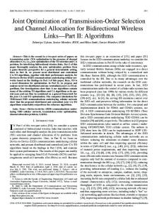
Fig. 2. The results from the simplified array image model. (a) Point spread function of the array inspection system shown as Fig. 1(a) at 9 different locations, (b) an example of the grain scatterer distribution in the test structure, note that the point reflector is at (0, 20), (c) the total focusing method (TFM) image generated by using the simplified model for Fig. 2(b) distribution, and (d) the rms image from the 100 simplified TFM image realizations.
1736
IEEE Transactions on Ultrasonics, Ferroelectrics, and Frequency Control ,
vol. 60, no. 8,
August
2013
Fig. 3. Parameter optimization for the forward scattering model. (a) SNR, ra, as a function of grain scatterer density, ρg, and (b) minimum number of realizations needed to generate the converged rms image as a function of scatterer density.
In the experiment, five 100-mm-thick samples of brass, steel, aluminum, and copper were chosen to represent materials with different degrees of back scattering. The defect detection capability of each imaging algorithm was demonstrated by imaging a 2-mm-diameter side-drilled-hole at 40 mm depth in these samples. An extra aluminum specimen with different types of defects was also chosen
to test imaging robustness, and is shown in Fig. 1(b). The specification of the array used in both simulation and experiment is described in Table I. Note that the sample geometries in the experimental samples are larger than those in simulation to reduce the effect of edge and back wall reflections.
Fig. 4. The results for assessing image resolution. (a) The total focusing method image for two point reflectors with the separation of 0.8 mm, (b) the comparison of image intensity distribution for two reflectors along the defect depth section (z = 20 mm) by using different image algorithms, and (c) the image intensity at the center of two point reflectors as a function of separation distance for different image algorithms.
zhang et al.: comparison of ultrasonic array imaging algorithms for nondestructive evaluation
1737
B. Parameter Optimization of the Hybrid Scattering Model
Fig. 5. The image comparison for different types of defect, i.e., a point reflector, a 3-mm-long horizontal crack and a 3-mm-long 45° inclined crack, in a structure without material backscattering, by using different image algorithms, (a) total focusing method, (b) phase-coherent imaging (PCI) with the factor FC, (c) PCI with the factor FS, and (d) spatial compounding imaging. Note that all figures are plotted in [−20 0] dB.
In the simulation, the full array data set for the specified inspection configuration of material with various grain (backscatter) structures was generated by using the hybrid scattering model under the single-scattering assumption (described in Section II). The backscattering amplitude from material is associated with the number of grain scatterers, ng, and the amplitude of a grain scatterer, Sg, which is related to a for a given Sd. Note that ng and a have opposite effects. Larger numbers of ng and low amplitudes of a can lead to strong backscattering. However, a larger number of ng also makes the computation time longer. The computation cost of the whole simulation procedure also depends on the number of realizations of scatterer positions, nr, which is required for the convergence of the whole simulation process. In this section, these parameters (ng, a, and nr) were optimized for efficient array data set generation. Fig. 2 shows an example of using the simplified array image model (11) to generate a defect image in a structure with strong backscatter. In this example, for a 40 × 40 mm copper structure (mx = mz = 40 mm, c = 4700 m/s, λ = 0.94 mm at 5 MHz), there are 5745 randomly distributed grain scatterers (ng = 5745, 5 scatterers per λ2, ρg = ng /(mx × mz) = 5/λ2) and a point reflector at (0, 20) that represents a target defect, and the scattering amplitude ratio of the point reflector to a grain scatterer is a = 8. Fig. 2(a) shows the PSF at 9 different locations for the specified array inspection configuration (Fig. 1 and Table I). A grain scatterer distribution function, D, is shown in Fig. 2(b). The final image, I, is the convolution of D and PSF (11), and is shown in Fig. 2(c). Note that in the convolution, the PSF at the position closest to a scatterer was used. Fig. 2(d) shows the rms image, Irms, from 30 grain scatterer distribution realizations. Note that the convergence of Irms from different number of scatterer distribution realizations indicates the convergence of the whole simulation process.
Fig. 6. Comparison of the weight factors used for different types of defect for (a) FC and (b) FS.
1738
IEEE Transactions on Ultrasonics, Ferroelectrics, and Frequency Control ,
There are several different SNR definitions used in the paper for different analysis purposes. For some imaging algorithms (specifically linear ones) it is legitimate to generate separate images for the target and noise because the final image is the superposition of the two. In this way, the actual SNR can be computed from the separate defect image, Id, without grain scatterers and the rms of separate grain noise images, Ig-rms, without defect, and is given by ra = q d/σ g , (13)
where qd is the peak amplitude at the defect location in Id, and σg is the rms of Ig-rms. However, for nonlinear imaging algorithms, the signals from a defect and those from grain scatterers cannot be separated in this manner, and the expected SNR must be computed from the final rms image, Irms, by r = q /σ, (14)
where q is the peak amplitude at the defect location in Irms, and σ is the rms of Irms in the region excluding the defect [marked as the region outside the 5 × 5 mm dashed box in Figs. 2(d)]. The SNR in each image realization, Ij, can also be extracted in the same way, and is given by
〈I n2(x, z )〉
S ≈ d a
Aρ g na
vol. 60, no. 8,
August
2013
na
∑ P(x, z, x i, z i) 2. (18) i =1
As na → ∞, A/na → dA = dx1 dz1 and the equation can be expressed as
〈I n2(x, z )〉 ≈
S d ρg a
∫∫
2
P(x, z, x 1, z 1) dx 1 dz 1. (19)
The expected rms noise amplitude at each pixel is therefore a function of ρ g . ρg and a can then be merged as a single parameter β by
β=
ρg . (20) a
This is similar to the figure of merit defined in [21]. In other words, the same image backscattering noise can be achieved using different scatter density as long as the ratio β is preserved. Computationally, it is more efficient for ρg
r j = q j /σ j , (15)
where the subscript j indicates the index of an image realization, qj is the peak amplitude at the defect location in Ij, and σj is the rms of Ij in the region excluding the defect [marked as the region outside the 5 × 5 mm dashed box in Fig. 2(c)]. It is also instructive to consider the minimum rj over all realizations: rmin = min(r j ). (16)
The convergence of the final rms images depends on the model area, mx × mz, the scatterer density, ρg, and the scattering amplitude ratio between the target defect and a grain scatterer, a. The expected rms noise amplitude at each pixel can be extracted from (12), and is 〈I n2(x, z )〉
=
Sd a
na
na
∑ ∑ 〈D(x i, z i)D(x j, z j )〉P(x, z, x i, z i)P *(x, z, x j, z j ). i =1 j =1
(17) Note that n 2 g when i ≠ j 〈D(x i, z i )D(x j, z j )〉 = n a and n g = Aρ g. n g when i = j n a Assuming ng/na ≫ (ng/na)2, (17) can be approximated as
Fig. 7. The image comparison for different types of defect in the structures with a = 11, by using different image algorithms, (a) total focusing method, (b) phase-coherent imaging (PCI) with the factor FC, (c) PCI with the factor FS, and (d) spatial compounding imaging. Note that all figures are plotted in [−20 0] dB.
zhang et al.: comparison of ultrasonic array imaging algorithms for nondestructive evaluation
1739
Fig. 8. Different SNRs (r and rmin) as a function of a for different types of defect: (a) a point reflector, (b) a 3-mm-long horizontal crack, and (c) a 3-mm-long 45° inclined crack.
to be as low as possible. Fig. 3(a) shows convergence of ra from 100 final image realizations (nr = 100) as a function of the scatterer density, ρg, at various β cases. From Fig. 3(a), it can be seen that when the scatterer density is greater than 5 scatterers per λ2 (ρg ≥ 5/λ2 and ng ≥ 5745), ra converges for all β cases. Fig. 3(b) shows the minimum number of realizations, nrm, needed to achieve convergence of ra. Convergence of ra is assumed when the number of realization is more than nrm, the difference of the rms images from nrm and all nr realizations, e, is less than 2%, where
∑x,z M ( n ∑j =1 I j2(x, z) ) 1
e=
1
n rm
rm
∑x,z M ( n ∑j =1 I j2(x, z) ) 1
1
nr
− 1 × 100%, (21)
r
where M is the total number of pixel in an image, (M = 1602). The lowest computation cost parameters ρg and nrm are taken at the beginning of convergence of simulation results. From Fig. 3, it can be seen that the lowest computation cost parameters for simulating the array data set to generate convergent rms images can be chosen as ρg = 5/λ2 and nrm = 15. On a standard desktop computer, it took 4 and 10 computational hours for models with 5745 and 11490 grain scatterers to generate array data sets, respectively.
C. Assessment of Imaging Algorithms The performance of all imaging algorithms was assessed by image resolution, image robustness to different types of defects in a structure, and image SNR. Note that all images were generated from the simulated full matrix data, and their plots are in decibels relative to their own peak amplitude. 1) Image Resolution: The image resolution for the different algorithms was investigated in a structure without material backscatter by imaging two closely-spaced point reflectors. Fig. 4(a) shows the TFM image for two point reflectors with a separation of 1.2 mm at a depth of 20 mm (z = 20). The image intensity distributions along the defect depth sections from the three different imaging algorithms (TFM, PCI, and SCI) were compared and are shown in Fig. 4(b). In Fig. 4(b), the results from PCI with the sign coherence factor (Fs) show the narrowest distribution and the lowest image intensity at the center (x = 0). This intensity is shown as a function of separation distance in Fig. 4(c). The image resolution can be defined as the shortest separation distance of two points that gives a specified threshold in image amplitude between them. For example, for a threshold of −3 dB, the resolutions for PCI with circular coherence factor and sign coherence factor
1740
IEEE Transactions on Ultrasonics, Ferroelectrics, and Frequency Control ,
vol. 60, no. 8,
August
2013
Fig. 9. The histogram of the image SNR, rj, from 100 grain distribution realizations at the cases of a = 5.5, 2.8, 1.4, 0.7, and for different types of defect: (a) a point reflector, (b) a 3-mm-long horizontal crack, and (c) a 3-mm-long 45° inclined crack.
are 0.52 mm and 0.51 mm, respectively, TFM resolution is 0.6 mm and SCI resolution is 0.7 mm. However, none of imaging algorithms can resolve point reflectors with a separation distance less than 0.5 mm (note that Rayleigh spatial resolution limit is 0.58 mm).
2) Image Robustness in a Structure Without Material Backscatter: The image robustness to different defect types was assessed by comparing images from structures without material backscatter. Fig. 5 shows a comparison of images for different types of defects (i.e., a point reflec-
Fig. 10. Experimental speckle images from different samples without defects by using the total focusing method image algorithm.
zhang et al.: comparison of ultrasonic array imaging algorithms for nondestructive evaluation TABLE II. Array Speckle Image Amplitude for Different Materials. Material Naval brass C4640 Stainless steel 304 Aluminum 6082 Mild steel 080A Copper C101
1741
TABLE III. SNR (in Decibels) for a Defect at 40 mm Deep in Different Materials Using Various Imaging Algorithms.
λ at 5 MHz (mm)
Irms in ROI1 (dB)
Irms in ROI2 (dB)
0.88 1.15 1.28 1.18 0.94
−4 0.1 0 2.3 3.8
−4.1 −1.6 −1.2 5 2
tor, a 3-mm-long horizontal crack and a 3-mm-long 45° inclined crack) obtained using TFM, PCI, and SCI. As shown in Fig. 5, PCI shows higher resolution, but suppresses the specular response of the 0° crack, which may lead to incorrect characterization of the defect. This is caused by variation in the PCI weighting function [Fc and Fs in (9) and (10)] along the crack specular surface. Fig. 6 shows Fc and Fs variations for different reflectors typical including a point reflector, a 3-mm-long crack, and an infinitely long interface at the same location (0, 20). As shown
Material Naval brass C4640 Stainless steel 304 Aluminum 6082 Mild steel 080A Copper C101
TFM
PCI (Fc)
PCI (Fs)
SCI
34 36 34 34 7
40 41 40 37 19
40 46 46 37 20
31 32 31 31 6
TFM = total focusing method; PCI = phase-coherent imaging; SCI = spatial compounding imaging.
in Fig. 6, the weighting function has smaller values at the specular reflector locations along the length of the crack than at the point reflector and crack tip locations. This is because the specular signal reflection points for different array element combinations occur at different points along the crack/interface. This results in different path lengths for different element pairs and, hence, higher phase variations.
Fig. 11. Experimental results from the 100-mm-thick samples with different back scatterers and a 2-mm side-drilled-hole at the depth of 40 mm by using a filter fc = 5 MHz and different image algorithms, (a) total focusing method, (b) phase-coherent imaging (PCI) with the factor FC, (c) PCI with the factor FS, and (d) spatial compounding imaging. Note that all figures are plotted in [−20 0] dB.
1742
IEEE Transactions on Ultrasonics, Ferroelectrics, and Frequency Control ,
vol. 60, no. 8,
August
2013
Fig. 12. Experimental results from the 100-mm-thick copper sample with a 2-mm side-drilled-hole at the depth of 40 mm by using various filters (fc = 3 to 7 MHz) and different image algorithms, (a) total focusing method, (b) phase-coherent imaging (PCI) with the factor FC, (c) PCI with the factor FS, and (d) spatial compounding imaging. Note that all figures are plotted in [−20 0] dB.
3) Image SNR and Robustness in a Structure With Material Backscatter: The image performance was first assessed by comparing an image realization from the structure with material backscatter, and then the image SNRs, r, rj, and rmin, were used to make an assessment. Fig. 7 shows a comparison of images from the structure with weak grain backscatter (a = 8). Comparing Figs. 5 and 7, it can be seen that PCI suppresses image noise at the expense of suppressing the specular response of the crack. The image SNR, rj, was then extracted from 15 random grain scatterer realizations with different a levels. Fig. 8 compares r and rmin from all three imaging algorithms for the simulated data with various a, and it directly indicates the defect detection capability of each imaging algorithm for NDE. For example, if choosing 6 dB for rmin as the detectable threshold, all three imaging algorithms show similar performance, and they can detect a point reflector in a structure with a > 3, a 3-mm-long horizontal crack in a structure with a > 3, and a 3-mmlong 45° inclined crack in a structure with a > 11. Note that it took 2160 computational hours (90 d) to generate each figure in Fig. 8 based on 30 realizations. By perform-
ing 20 parallel computations using a high-performance computing facility (Bristol Blue Crystal at the University of Bristol), the actual computation time is 4 d. Fig. 9 shows the histograms from 100 realizations for the different defects in the structures with a = 4, 2, 1, and 0.5. In Fig. 9, it can be seen that, compared with the other two imaging algorithms, the results from TFM show the most concentrated distribution in all cases. This indicates the most consistent imaging performance. From Figs. 8 and 9, it can be seen that a higher SNR can be achieved by using PCI for a structure with weak material backscatter. However, for a structure with strong material backscatter, the performance of all three imaging algorithms is similar. D. Experimental Results It is difficult to quantitatively validate the presented scattering model because of the difficulty of measuring grain size and its distribution in material. Moreover, the purpose of the paper is to investigate the relative imaging performance from different algorithms. In this case,
zhang et al.: comparison of ultrasonic array imaging algorithms for nondestructive evaluation
Fig. 13. The experimental image performance indicated by SNR as a function of the filter central frequency for different image algorithms.
it is not necessary to know accurately the material parameters that control the back scattering amplitude, and the experiments are focused on generating defect images with different SNR levels, particularly at high SNR levels. The material speckle patterns of 5 different materials with sample dimensions 100 × 300 × 30 mm (brass, stainless steel, aluminum, mild steel, and copper) were first measured. A 2-mm-diameter side-drilled-hole was then drilled at 40 mm depth in these samples to use to test the detection capability of each imaging algorithm. For the copper sample, the same array data set processed by filters with
1743
different center frequencies was used and assumed to be equivalent to the data from structures with various a. The robustness of different imaging algorithms was finally tested using several different defects in an aluminum sample. Fig. 10 shows TFM speckle images of different material without defect using the 5-MHz array (details shown in Table I). The images are plotted on a decibel scale and normalized to the rms amplitude in the aluminum image satisfying |x| ≤ 20 mm and 10 ≤ z ≤ 30 mm. This 20 × 20 mm region of interest is henceforth denoted ROI1, and is shown by the rectangle in Fig. 10. RMS speckle amplitude values in ROI1, Irms, are given in Table II along with the ultrasonic wavelength, λ, at 5 MHz for different materials tested. Also listed in Table II is the rms speckle amplitude values in ROI2, satisfying |x| ≤ 20 mm and 30 ≤ z ≤ 50 mm. Except for the mild steel sample, all other samples show reduced amplitude in ROI1, and this is caused by the scattering from the grain structure [19], [20]. The larger amplitude in ROI2 from the mild steel sample is believed to be caused by larger grains at 40 mm depth. Fig. 11 shows the image comparison from different materials using different imaging algorithms for a 2-mmdiameter side-drilled-hole at a depth of 40 mm in each sample. The full array data set was first processed using filters at center frequencies, fc = 5 MHz, and the processed data sets were then used to generate images. As
Fig. 14. Experimental results from the aluminum sample [Fig. 1(b)] by using different image algorithms, (a) total focusing method, (b) phasecoherent imaging (PCI) with the factor FC, (c) PCI with the factor FS, and (d) spatial compounding imaging.
1744
IEEE Transactions on Ultrasonics, Ferroelectrics, and Frequency Control ,
shown, the defect is visible in brass, aluminum, and steel, and PCI suppresses image noise, but the defect is indistinguishable from surrounding signals in copper in TFM images. The rj from each defect image is listed in Table III; the copper sample shows the lowest SNR level. The copper sample was then further used to test the capability of defect detection by generating the images with different SNR levels. Fig. 12 shows the images obtained using filters with fc from 3 to 7 MHz and different imaging algorithms. As shown, when using filters with fc ≤ 5 MHz, the defect is visible in all images and PCI suppresses image noise, but the defect is indistinguishable from surrounding signals when using the filters with fc > 5 MHz. Fig. 13 shows the extracted SNR, as a function of fc. Again, the PCI has a better SNR for a structure with weak material backscatter, and all imaging algorithms show similar performance when material backscatter becomes strong. This agrees with the simulated results shown in Fig. 8. The resolution improvement from PCI is demonstrated by the point reflector images in Fig. 14 for the aluminum sample. However, compared with the TFM and SCI images [Figs. 14(a) and 14(d)], the PCI image [Figs. 14(b) and 14(c)] for the planar defect shows lower amplitude and discontinuity along the length of the defect. This may lead to misleading defect characterization.
V. Conclusions A procedure for qualitatively and quantitatively assessing the relative performance of imaging algorithms was developed. This includes a hybrid forward scattering model for randomly distributed grain scatterers and the following performance indicators: image resolution, SNR and robustness. The performance of three widely-used imaging algorithms (TFM, PCI, and SCI) was examined through both simulation and experimental measurements. It was demonstrated that PCI can yield higher image resolution than the TFM for structures with weak material backscatter, but that the weight factors for PCI images should be chosen carefully to avoid image distortion. Overall, the TFM is the most robust algorithm for different types of defects. It was also shown that the detection limit of all three imaging algorithms is similar for weakly scattering defects. The procedure of assessing imaging performance described in the paper can also be used for the assessment of other imaging algorithms.
References [1] B. W. Drinkwater and P. D. Wilcox, “Ultrasonic arrays for nondestructive evaluation: A review,” NDT Int., vol. 39, no. 7, pp. 525– 541, 2006. [2] R. Ahmad, T. Kundu, and D. Placko, “Modeling of phased array transducers,” J. Acoust. Soc. Am., vol. 117, no. 4, pt. 1, pp. 1762– 1776, 2005.
vol. 60, no. 8,
August
2013
[3] S. Mahaut, O. Roy, C. Beroni, and B. Rotter, “Development of phased array techniques to improve characterization of defect located in a component of complex geometry,” Ultrasonics, vol. 40, no. 1–8, pp. 165–169, 2002. [4] M. G. Lozev, R. L. Spencer, and D. Hodgkinson, “Optimized inspection of thin-walled pipe welds using advanced ultrasonic techniques,” J. Press. Vessel Technol., vol. 127, no. 3, pp. 237–243, 2005. [5] N. Portzgen, D. Gisolf, and G. Blacquiere, “Inverse wave field extrapolation: A different NDI approach to imaging defects,” IEEE Trans. Ultrason. Ferroelectr. Freq. Control, vol. 54, no. 1, pp. 118– 127, 2007. [6] C. Holmes, B. W. Drinkwater, and P. D. Wilcox, “Post-processing of the full matrix of ultrasonic transmit-receive array data for nondestructive evaluation,” NDT Int., vol. 38, no. 8, pp. 701–711, 2005. [7] A. J. Hunter, B. W. Drinkwater, and P. D. Wilcox, “The wavenumber algorithm for full-matrix imaging using an ultrasonic array,” IEEE Trans. Ultrason. Ferroelectr. Freq. Control, vol. 55, no. 11, pp. 2450–2462, 2008. [8] A. Velichko and P. D. Wilcox, “An analytical comparison of ultrasonic array imaging algorithms,” J. Acoust. Soc. Am., vol. 127, no. 4, pp. 2377–2384, 2010. [9] G. E. Trahey, S. W. Smith, and O. T. Von Ramm, “Speckle pattern correlation with lateral aperture translation: Experimental results and implications for spatial compounding,” IEEE Trans. Ultrason. Ferroelectr. Freq. Control, vol. 33, no. 3, pp. 257–264, 1986. [10] P. M. Shankar, “Speckle reduction in ultrasound B-scans using weighted averaging in spatial compounding,” IEEE Trans. Ultrason. Ferroelectr. Freq. Control, vol. 33, no. 6, pp. 754–758, 1986. [11] P. Chaturvedi, M. F. Insana, and T. J. Hall, “2-D companding for noise reduction in strain imaging,” IEEE Trans. Ultrason. Ferroelectr. Freq. Control, vol. 45, no. 1, pp. 179–191, 1998. [12] A. Gerig, T. Varghese, and J. A. Zagzebski, “Improved parametric imaging of scatterer size estimates using angular compounding,” IEEE Trans. Ultrason. Ferroelectr. Freq. Control, vol. 51, no. 6, pp. 708–715, 2004. [13] J. Camacho, M. Parrilla, and C. Fritsch, “Phase coherence imaging,” IEEE Trans. Ultrason. Ferroelectr. Freq. Control, vol. 56, no. 5, pp. 958–974, 2009. [14] J. Camacho and C. Fritsch, “Phase coherence imaging of grained materials,” IEEE Trans. Ultrason. Ferroelectr. Freq. Control, vol. 58, no. 5, pp. 1006–1015, 2011. [15] Z. Torbatian, R. Adamson, M. Bance, and J. A. Brown, “A splitaperture transmit beamforming technique with phase coherence grating lobe suppression,” IEEE Trans. Ultrason. Ferroelectr. Freq. Control, vol. 57, no. 11, pp. 2588–2595, 2010. [16] J. A. Johnson, M. Karaman, and B. T. Khuri-Yakub, “Coherent-array imaging using phased subarrays. Part I: Basic principles,” IEEE Trans. Ultrason. Ferroelectr. Freq. Control, vol. 52, no. 1, pp. 37–50, 2005. [17] J. Zhang, B. W. Drinkwater, P. D. Wilcox, and A. Hunter, “Defect detection using ultrasonic arrays: The multi-mode total focusing method,” NDT Int., vol. 43, no. 2, pp. 123–133, 2010. [18] A. Velichko and P. D. Wilcox, “Strategies for ultrasound imaging using two dimensional arrays,” Rev. Prog. QNDE, vol. 29, pp. 887–894, 2010. [19] L. W. Schmerr, Fundamentals of Ultrasonic Nondestructive Evaluation—A Modeling Approach. New York, NY: Plenum Press, 1998. [20] I. Yalda, F. J. Margetan, and R. B. Thompson, “Predicting ultrasonic grain noise in polycrystals: A Monte Carlo model,” J. Acoust. Soc. Am., vol. 99, no. 6, pp. 3445–3455, 1996. [21] F. J. Margetan, R. B. Thompson, and I. Yaldamooshabad, “Modeling ultrasonic microstructural noise in titanium-alloys,” Rev. Prog. QNDE, vol. 12B, pp. 1735–1742, 1993. [22] P. D. Wilcox, “Array imaging of noisy materials,” Rev. Prog. QNDE, vol. 30, pp. 890–897, 2011. [23] F. G. Miller and H. Pursey, “The field and radiation impedance of mechanical radiators on the free surface of a semi-infinite isotropic solid,” Proc. R. Soc. Lond., vol. 223, no. 1155, pp. 521–541, 1954. [24] J. Zhang, B. Drinkwater, and P. Wilcox, “Defect characterization using an ultrasonic array to measure the scattering coefficient matrix,” IEEE Trans. Ultrason. Ferroelectr. Freq. Control, vol. 55, no. 10, pp. 2254–2265, 2008. [25] A. Velichko and P. D. Wilcox, “A generalized approach for efficient finite element modelling of elastodynamic scattering in two and three dimensions,” J. Acoust. Soc. Am., vol. 128, no. 3, pp. 1004–1014, 2010.
zhang et al.: comparison of ultrasonic array imaging algorithms for nondestructive evaluation Jie Zhang was born in Baoji, P. R. China in 1975. He received B.Eng., M. Eng., and Ph.D. degrees in instrument science and technology from the Harbin Institute of Technology (HIT), P. R. China, in 1997, 1999, and 2002, respectively. From 2002 to 2003, he was employed as a research fellow in the University of Warwick. Since 2003, he has worked as a research associate at the University of Bristol, and his current research interests are focused on ultrasonic NDE of layers, interfaces, ultrasonic wave scattering, and adaptive array imaging.
Bruce W. Drinkwater was born in Hexham, England, in 1971. He received the B.Eng. and Ph.D. degrees in mechanical engineering from Imperial College, London, England, in 1991 and 1995, respectively. His Ph.D. thesis was on the subject of dry-coupled ultrasonic devices for nondestructive evaluation (NDE). From 1996 to the present, he has worked as an academic in the Department of Mechanical Engineering at the University of Bristol, England. Between 2000 and 2005, he was awarded an EPSRC Advanced Research Fellowship, and in 2007, he was promoted to Professor. His research interests focus on ultrasonic NDE. He has published more than 100 articles on NDE of adhesive joints, thin layers, and interfaces, and ultrasonic sensing and imaging using arrays and guided waves, as well as particle manipulation for biological applications. Prof. Drinkwater is a member of the Institute of Mechanical Engineers, the British Institute of Non-Destructive Testing, and the American Society of Acoustics.
1745
Paul D. Wilcox was born in Nottingham, England, in 1971. He received an M.Eng. degree in engineering science from the University of Oxford, England, in 1994 and a Ph.D. degree from Imperial College, London, England, in 1998. From 1998 to 2002, he was employed as a research associate in the Non-Destructive Testing Research Group at Imperial College, where he worked on the development of guided wave array transducers for large area inspection. In 2002, he was appointed as a lecturer in the Department of Mechanical Engineering at the University of Bristol, England, and was promoted to professor in 2010. Dr. Wilcox was recently awarded an EPSRC Advanced Research Fellowship, and his current research interests include guided-wave structural health monitoring, elastodynamic scattering, and signal processing.