1932
IEEE Transactions on Ultrasonics, Ferroelectrics, and Frequency Control ,
vol. 56, no. 9,
September
2009
Ultrasonic Imaging Algorithms With Limited Transmission Cycles for Rapid Nondestructive Evaluation Ludovic Moreau, Bruce W. Drinkwater, and Paul D. Wilcox Abstract—Imaging algorithms recently developed in ultrasonic nondestructive testing (NDT) have shown good potential for defect characterization. Many of them are based on the concept of collecting the full matrix of data, obtained by firing each element of an ultrasonic phased array independently, while collecting the data with all elements. Because of the finite sound velocity in the test structure, 2 consecutive firings must be separated by a minimum time interval. Depending on the number of elements in a given array, this may become problematic if data must be collected within a short time, as it is often the case, for example, in an industrial context. An obvious way to decrease the duration of data capture is to use a sparse transmit aperture, in which only a restricted number of elements are used to transmit ultrasonic waves. This paper compares 2 approaches aimed at producing an image on the basis of restricted data: the common source method and the effective aperture technique. The effective aperture technique is based on the far-field approximation, and no similar approach exists for the near-field. This paper investigates the performance of this technique in near-field conditions, where most NDT applications are made. First, these methods are described and their point spread functions are compared with that of the Total Focusing Method (TFM), which consists of focusing the array at every point in the image. Then, a map of efficiency is given for the different algorithms in the nearfield. The map can be used to select the most appropriate algorithm. Finally, this map is validated by testing the different algorithms on experimental data.
I. Introduction
R
ecently, imaging techniques using ultrasonic phased arrays have been investigated in the field of nondestructive testing (NDT) [1], [2]. Most of them were developed in other areas such as medicine (total focusing method [3]), sonar (wavenumber algorithm [4]), or radar (synthetic aperture radar [5]), and have successfully been adapted to NDT applications. The recent interest in arrays among the NDT community is mainly because of their ability to produce 2-D and even 3-D images of a flaw with good accuracy. Considering a particular phased array designed to operate at a given frequency, the quality of the image produced depends, among other things, on both the size of its aperture and the choice of the imaging algorithm. In sonar-like applications, the synthetic aper-
Manuscript received March 6, 2009; accepted May 13, 2009. This work was funded by the Engineering and Physical Sciences Research Council, United Kingdom (Grant number EP/C534824). The authors are with the Department of Mechanical Engineering, University of Bristol, Bristol, UK (e-mail:
[email protected]). Digital Object Identifier 10.1109/TUFFC.2009.1269 0885–3010/$25.00
ture is increased by moving the source, which is known as the synthetic aperture focusing technique [6] (SAFT). However, this paper concerns static arrays only, although the results presented can be extended to moving arrays. Therefore, the aperture is fixed by the size of the array, thus making the choice of an appropriate algorithm crucial. Imaging algorithms can take advantage of the large number of possible transmit-receive combinations, because each firing contributes to reducing unwanted artifacts in the image, such as sidelobes [7]. The largest amount of information that can be gathered about a given defect with a fixed ultrasonic phased array is obtained when all elements are used separately as transmitters and receivers. If the array has N elements, then a maximum of N2 timetraces can be collected, which is known as the full matrix of transmit-receive data [8]. However, because of the finite time-of-flight of the ultrasonic waves in the medium, 2 consecutive firings must be separated by a minimum time interval. This introduces a minimum time required to capture the full matrix of data that is dependent on the number of independent firings. Typical acquisition times are given in Section IV, in which experimental results are presented. In an industrial context, it may not be possible to collect the full matrix because of shortened acquisition times, as is the case in high-speed rail inspections [9], for example. In such cases, there is a requirement to adapt the algorithms to produce an image with reasonable accuracy on the basis of an incomplete matrix of data because of the reduced number of firings. Similar problems occur in other areas such as medicine, because of blood flow or organ motion (heartbeat, breathing, etc.), and in the area of radar, where targets are generally not static. In an attempt to produce the best image for a given number of firings, a specific number of transmitters and/ or receivers can be chosen instead of all of them. The common source method (CSM) uses all elements to transmit simultaneously, so that a plane wave propagates into the structure and an image is created from the scattered waves [10]. Other approaches are based on defining arrays sparsely populated on transmit and generally fully populated (although not necessarily) on receive. In such approaches, a given number of transmitting and/or receiving elements are selected among the N elements of the array. However, the design of the best sparse array is still an ongoing research topic [11]. The solution considered in this paper is to define an effective aperture [12]. This
© 2009 IEEE
moreau et al.: imaging algorithms with limited transmission cycles
1933
Fig. 1. Data acquisition process for (a) full matrix capture, (b) common source method, and (c) sparse array.
consists of applying weighting functions to the transmitted and received signals, to compensate for the loss of data relative to the full matrix. It is based on the fact that, in the far-field of the array, redundancies exist in the full matrix of data. The aim of this work is to apply these 2 solutions (i.e., the CSM and the effective aperture technique) to NDT problems to test their performance, and classify the algorithms in terms of efficiency. The effective aperture compensation technique relies on the far-field approximation, but most NDT applications are in near-field conditions. Because no similar approach exists for the near-field, it is of interest to study the behavior of this technique when the inspection is made in the near-field of the array. Because both direction and distance from the array may influence the accuracy of the images in the near-field, different areas of inspection are studied, so that it becomes possible to choose a priori the most efficient algorithm to achieve a given level of accuracy. To classify them, their point spread functions (PSFs) are numerically calculated and compared with that generated with the total focusing method applied to the full matrix of data. In the last section, 2 experimental cases are presented. The first one consists of a simple configuration in which crossed-drilled holes are imaged in a steel sample. The second case is a more realistic situation, in which both crossed-drilled holes and a slot are imaged in an aluminum sample. II. Imaging Algorithms This section describes the different algorithms considered in this paper which are aimed at generating an image of the interior of a structure. It is assumed that a 1-D array is used to capture a set of data consisting of all possible transmit-receive combinations. First, the TFM is described. This algorithm will be used to produce reference images for the other techniques: the CSM and the sparse-TFM. Sparse-TFM is the term used to describe the case when the TFM algorithm is used to post-process
an incomplete matrix of data (i.e., obtained with a sparse transmit and/or receive aperture). This should not be confused with the sparse array image algorithm used in guided wave structural health monitoring [13]. A. Total Focusing Method Algorithm The TFM is an algorithm used to post-process the full matrix of ultrasonic transmit-receive array data. The principle of this technique is to focus the array at every point in the inspected region, for all combinations of elements, so that an image of this region can be produced. Originally used in the medical field [3], this method has successfully been used for NDT. Because a description of this method [10] and a study of its performance [8], [14] have already been detailed in the literature, only the algorithm is recalled in this section. Consider the 2-D configuration of a linear ultrasonic array with N elements, centered at the origin of the coordinate system (O, X, Y). X and Y are unit vectors parallel and orthogonal to the array face, respectively. The intensity of the TFM image I(r) at any point of the scanned area is given by: æ r - r T j + r - r R j¢ ç s j, j ¢ ççè c j =1 j ¢ =1 N
I (r) =
N
åå
ö÷ ÷÷, ø
(1)
where c is the wave velocity in the propagation medium, r is the position vector of the image point, rTj and rRj′ are vectors defining the positions of transmitter j and receiver j′, respectively. sj, j′ is the temporal signal received by receiver j′ when transmitter j is firing. As can be seen from (1), N 2 time-traces are used to produce the image. This set of data is called the full matrix. The acquisition process is illustrated in Fig. 1(a): separately, each element of the array sends an ultrasonic signal into the structure, and all receivers collect the scattered signals. Depending on the time-of-flight of these signals and the hardware used, the acquisition of the full
IEEE Transactions on Ultrasonics, Ferroelectrics, and Frequency Control ,
1934
matrix can be time consuming. Note that the full matrix is symmetric because of reciprocity, then only N(N + 1)/2 time-traces are unique, but this does not reduce the number of required transmission cycles, and thus has no effect on the speed of the full matrix capture. B. The Common Source Method This method consists of collecting the data with each receiver, when all elements of the array transmit simultaneously [Fig. 1(b)]. Its main advantage is that only one firing is required, thus making this algorithm the most efficient in terms of imaging speed. It also allows more energy to be input in the media. As with the TFM algorithm, this technique is based on the evaluation of the time-of-flight between the scatterer and the elements. However, only N time-traces are used for the image construction, and this has a detrimental effect on image performance. This algorithm is described in the following equation: æ r.Y + r - r R j ¢ ç I (r) = s j ¢ ççè c j ¢ =1 N
å
ö÷ ÷÷, ø
(2)
where sj′ is the temporal signal received by receiver j′.
I (r) =
æ r - r T j + r - r R j¢ ç s j, j ¢ ççè c j Î[T ] j ¢ Î[R]
åå
ö÷ ÷÷, ø
(3)
where [T] denotes the set of transmitters and [R] that of receivers selected in the sparse transmit and receive apertures, respectively. Therefore this algorithm is similar to the TFM algorithm, but not all combinations of transmitters and/or receivers are used in the imaging process. As the current work is motivated by the desire to minimize acquisition time by reducing the number of transmit cycles, only the case of a sparse transmit aperture and a full receive aperture is considered, as illustrated in Fig. 1(c). Moreover, to maximize the reduction of the data acquisition times, sparse transmit apertures where only 2 (i.e., dim([T]) = 2 and [R] = [1, …, N]) or 4 (i.e., dim([T]) = 4 and [R] = [1, …, N]) elements are fired are considered. The main difficulty when using a sparse transmit aperture comes from an under-sampling in the spatial domain, which results in grating lobes in the transmitted field [15].
2009
2) Far-Field Expression of the Point Spread Function: It is common to characterize the performance of an imaging algorithm by evaluating its point spread function (PSF), which is its response to a point-like target. In general, the wider the array aperture, the smaller the PSF, because the focusing becomes better [15], [16]. An exact expression for the PSF of an array can be obtained in the far-field, using appropriate far-field approximations. Consider a point-like scatterer in the inspected media, the position of which is defined by vector r0. In a 2-D homogeneous medium, both the field incident on the scatterer caused by a point transmitter at rT and the scattered field received at point rR at a particular frequency ω, can be approximated for the longitudinal wave in far-field conditions with a Green’s function of the form: g X (r 0, r X) =
C. Sparse-TFM Algorithms
1) Uncorrected Sparse-TFM Algorithm: The uncorrected sparse-TFM algorithm is defined by
September
An ideal distribution of elements satisfies the spatial Nyquist criteria in a given material, (i.e., a ≤ λ/2, where a is the element pitch and λ is the wavelength of the acoustic wave). For example, for the typical case of the inspection of aluminum at 5 MHz, the element pitch must be less than 0.63 mm to satisfy Nyquist criteria. In a media with smaller sound velocity (or for a greater frequency), this pitch has to be reduced.
The term sparse-TFM is used in this paper to refer to any algorithm designed to produce an image from an incomplete matrix of transmit-receive data, obtained when not all elements have been used as transmitters and/or receivers.
vol. 56, no. 9,
A r0 - rX
1/2
e ik r 0 - r X e -iwt,
(4)
where A is a constant, k is the wavenumber of longitudinal waves at frequency ω, t is time, and subscript X = T or R refers to transmission or reception. In subsequent expression the e−iωt is omitted for brevity. The principle of delay-and-sum algorithms such as the TFM, sparse-TFM or CSM is to invert the phase of the Green’s function, to calculate the amplitude of the scattered signal at the image point, r, at an instant corresponding to the corresponding time of propagation in the media. This is achieved by applying phase shifts of the form:
f X (r X, r) = e -ik r X - r ,
(5)
where again the subscript X = T or R refers to phase shifts calculated for the incident wave (fT) or the scattered wave (fR), respectively. In the far-field of the array, |r|,|r0| ≫ |rT|,|rR|. Therefore, by using the approximation
a-e » a -
a.e , a
(6)
where a and e are 2 vectors such as |a| ≫ |e|, (4) and (5) can be written as: and
g X (r 0, r X) »
A r0
1/2
e ik r 0 e -((ikr 0)/ r 0 )r X
(7)
moreau et al.: imaging algorithms with limited transmission cycles
i(r 0, r) »
A 2e 2ik( r 0 - r ) r0
ò¥e
((-ikr)/ r )r T ((ikr 0)/ r 0 )r T
e
f X (r X, r) » e -ik r e ((ikr)/ r )r X.
u(r T)w T (r T)dr T
(8)
To describe the array element positions in the transmit and receive apertures, the binary valued functions u and v of position r are used. These functions are unity at the spatial location of the transmitter/receiver and zero elsewhere. Functions wT and wR represent transmit and receive weighting functions applied to u and v, to control the relative contribution of each element to the image. The PSF, which includes the contribution from all transmit-receive element pairs, can then be expressed as the following double integral:
i(r 0, r) =
ò ò¥ g T (r 0, r T)f T (r T, r)u(r T)w T (r T) × g R(r 0, r R)f R(r R, r)v(r R)w R(r R)dr Tdr R.
(9)
Substituting (7) and (8) into (9) results in (10), see above. By performing the change of variables b = k(r/|r|) and b0 = k(r0/|r0|), the integrals can be recognized as spatial Fourier transforms in the b domain of the transmit and receive apertures defined by:
AT (b) =
+¥
ò-¥ u(r T)w T (r T)e ibr dr T, T
(11)
and
A R(b) =
+¥
ò-¥ v(r R)w R(r R)e ibr dr R. R
(12)
Consequently, in the far-field of the array, the PSF can be evaluated by calculating the product between these 2 apertures, in the b domain:
i(r 0, r) »
2 2ik( r 0 - r )
Ae
r0
AT (b - b 0) × A R(b - b 0). (13)
This equation remains valid for all r and r0 as long as as |r|, |r0| ≫ |rT|, |rR|. 3) Corrected Sparse-TFM Algorithm: This section presents a method used to remove unwanted image artifacts caused by the use of a sparse transmit or receive aperture, by applying appropriate apodization coefficients to transmit and/or receive signals. If the product AT ∙AR in (13) is defined as Aar, then the inverse spatial Fourier transform aar of Aar is the spatial convolution of u∙wT and v∙wR:
1935
a ar(r) = u(r)w T (r) Ä v(r)w R(r),
(14)
ò¥e
((-ikr)/ r )r R ((ikr 0)/ r 0 )r R
v(r R)w R(r R)dr R
e
(10)
which is known as the effective aperture of the array. Consequently, any pair of u∙wT and v∙wR that convolve to give the same result will have the same PSF in the far-field [17], [18]. Therefore, the fundamental idea of the effective aperture correction is to apply weighting functions to the transmit and received data from a sparse array, so that it has the same effective aperture as a fully populated array. Under far-field conditions, these sparse and fully populated arrays have the same PSF, and the artifacts caused by the sparse aperture are removed. To reduce the number of firings for increased speed of imaging, the effective aperture can be used to design an array with a sparse transmit aperture that has the same performance as an array with a full transmit aperture. In the following, this will be referred to as the effective aperture correction. To apply the effective aperture correction, we consider 2 arrays denoted by I and II. Array I is fully populated and no correction is applied to its data (i.e., wT = wT = 1) and array II has sparse transmit and/or receive apertures. When the effective aperture correction is used, the weighting functions are chosen so that they compensate for the lack of elements. In that case, they must be such that:
u I (r) Ä v I (r) = (w T (r) × u II (r)) Ä (w R(r) × v II (r)). (15)
In practice, the elements of [T] transmit at different times, to create the synthetic aperture. The total effective SA aperture a ar is then the sum of all the effective apertures resulting from these independent firings:
SA a ar (r) =
Nf
å(u m(r)w Tm(r)) Ä (v m(r)w Rm(r)).
(16)
m =1
In this equation, Nf is the number of independent firings, and um and vm are the functions defining the distribution of the transmit and receive elements at firing m, apodized with weighting functions w Tm and w Rm, respectively. Once the desired effective aperture has been chosen for an array with sparse transmit and/or receive apertures, the effective aperture correction is used in the sparse-TFM algorithm by implementing the apodization functions: I (r) =
æ r - r T j + r - r R j ¢ ö÷ ÷÷ . ø c
ç w Tj (r)w Rj(r)s j, j ¢ ççè åå ¢
j Î[T ] j Î[R]
(17) Because (16) has Nf unknown functions of both w Tm and (2Nf in total), there are an infinite number of ways to define these weighting functions. This means that any set
w Rm
1936
IEEE Transactions on Ultrasonics, Ferroelectrics, and Frequency Control ,
vol. 56, no. 9,
2009
September
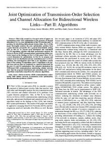
Fig. 2. Far-field point spread function calculated with (a) total focusing method (TFM) algorithm, (b) uncorrected 2-firings sparse-TFM algorithm, (c) 2-firings sparse-TFM algorithm corrected with triangle effective aperture, and (d) 2-firings sparse-TFM algorithm corrected with Gaussian effective aperture.
of functions wT and wR that satisfies (16) will make the corrected sparse-TFM algorithm produce the same image in the far-field. For implementation convenience, the following analysis considers the apodization of only the receive data by setting wT(rT) = 1, for all rT, and adapting the functions w Rj. Fig. 2 shows the simulated far-field PSF of a 64-element array when 4 different combinations of transmit and receive apertures are considered. In the first case, a fully populated array is used, thus allowing the TFM algorithm to produce the image [Fig. 2(a)]. In the other cases, only the edge elements (i.e., the 1st and the 64th) act as transmitters, while all elements are used to collect the data [Figs. 2(b) and (c)]. The PSFs were calculated by considering the propagation of longitudinal waves in aluminum at 5 MHz (λ = 1 mm). The PSF of the uncorrected sparse-TFM algorithm is significantly different from that of the TFM, and sidelobes appear at −15 dB [Fig. 2(b)] because of the effective aperture resulting from the transmit and receive apertures. However in the third case, apodization coefficients have been applied to received data to correct the sparse-TFM algorithm as shown graphically in the figure. Eq. (16) states that 2 sets of coefficients are necessary, because 2 firings are made. In that case, a convenient way of defining these coefficients is given by:
w R(1) = f (N )/2, and w R(j) = f (j - 1 + N /2),
j Î [2,..., N ],
(18)
for the first firing, and w R(N ) = f (N )/2, and w R(j) = f (j), j Î [1,..., N - 1],
(19)
for the second one. f is the shape of the desired effective SA aperture a ar , defined for j ∈ [1, …, 2N – 1]. To produce a triangular effective aperture, the coefficients are represented in Fig. 2(c). This effective aperture is identical to that of an array fully populated on transmit and receive without apodization [Fig. 2(a)], and is given by: SA a ar (r)
Nf
=
å(P N f /2(x - (N f /2 + 1))) Ä (d(x - m))
m =1 Nf
=
åP N f /2(x - (N f /2 + 1) - m),
m =1
(20)
where P N f /2 is the boxcar function with width Nf/2. ConSA sequently, a ar is the effective aperture naturally generated when using the TFM algorithm, where no apodization is used either in transmit or receive. By comparing Figs. 2(a) and (c), it can be seen that the resultant PSF is exactly the same. The triangular effective aperture produces sidelobes that first appear at −27 dB [Fig. 2(a) and (c)]. An additional apodization with a Gaussian shape is now implemented, which further reduces the level of the first sidelobes to
moreau et al.: imaging algorithms with limited transmission cycles
−32 dB [Fig. 2(d)]. In this paper, the authors will consider an image to be of acceptable quality if sidelobes have a level below −30 dB, which is a representative dynamic range of many industrial applications. In an image presented on a 30 dB dynamic range, this will avoid sidelobe artifacts, but on the other hand will also make the main lobe of the PSF slightly larger than that of the triangular effective aperture. Note that the criteria of a sidelobe level below −30 dB is arbitrary and the choice of effective aperture shape depends on the characteristics required in the final image. For a detailed comparison of different effective apertures’ efficiency, the reader can refer, for example, to [19]. In the following, to make results comparable between the sparse-TFM and TFM algorithms, these 2 algorithms both receive a Gaussian effective aperture correction. The use of apodization functions to modify the effective aperture of an array relies on the far-field approximation. However, many NDT applications with arrays are in nearfield conditions. As far as the authors are aware, no similar analysis exists for the near-field, because the physical requirements to apply the effective aperture theory in the near-field cannot be satisfied. Recently, beamforming has been investigated in the near-field of the array with a sparse transmit aperture, using the broadband minimum variance theory [20]. It requires weighting functions to be applied for each pair of transmit-receive elements and at each point in the image. However, these data-dependent coefficients make the algorithm non-deterministic and may lead to instability. This illustrates the complexity of designing a sparse array to image in both near- and farfields. Consequently, it is of interest to explore the performance of the effective aperture correction technique in the near-field of the array. III. Near-Field Performance of Algorithms In this section, point-like defects are simulated in aluminum using an analytical model. Only longitudinal waves are considered in the simulations, with speed equal to 6100 m/s. This model uses the minimum time-of-flight of the acoustic signals between the elements of the array and the target, which is used in turn to calculate a phase shift in the temporal waveform. To simulate signals generated with a 5-MHz phased array, again with 64 elements on a 0,63 mm pitch, the input signal is chosen to be a 2.5-cycle toneburst of central frequency 5 MHz, with a Gaussian window. Because the position of the point-like target with respect to the center of the array may have an influence on the results, several directions of inspection are considered. They are defined by the angle θ, measured from the normal to the array surface. For each position of the reflector, the PSF is calculated with the CSM and the sparse-TFM algorithms (both with and without effective aperture correction), and compared with the point spread function of the TFM. Five directions of inspection are considered: θ = 0, 10, 20, 30, and 45°. For each direction, the position of
1937
the target is varied from 10 mm to 100 mm away from the center of the array, in steps of 10 mm. If D denotes the aperture of the array, then the distance to reach the far-field is of the order D 2/λ. For the 64-element array D = 40 mm, λ = 1.22 mm, and the ratio D 2/λ is equal to 1.33 m. Therefore, all the positions considered are in the near-field of the array. The TFM is used as the reference algorithm for this study, although some other techniques may produce slightly better images [21]. For the comparison of the algorithms, the following factor is defined:
D=
API alg - API TFM , API TFM
(21)
where API is the array performance indicator [8]. This factor measures the area where the intensity of the PSF is greater than a given dB value related to its maximum value. For the API to be calculated accurately, a pixel size of 0.25 mm has been chosen in all images. In (21), subscript alg denotes the algorithm used to calculate the API values. Factor Δ is therefore the relative image quality between a specific algorithm and the TFM algorithm. As indicated previously, a 30 dB dynamic range is considered to be a reasonable target level of accuracy for this study. Consequently API and Δ values are calculated by taking into account all pixels having an intensity greater than −30 dB. This means that both the PSF and imaging noise will contribute to the comparison of the algorithms. Fig. 3 shows the PSF calculated for both the TFM (right-hand side) and the corrected 4 firings sparse-TFM (left-hand side) when θ = 0, at 3 different distances from the array: 10, 30, and 50 mm. The figure shows the different levels of thresholds of the PSF, and it can be seen that the images produced by these 2 algorithms become more similar as the distance between the array and the target increases. Such images were calculated for all algorithms and positions considered in this study, to calculate Δ and to plot Fig. 4, in which the algorithms are compared. When comparing the algorithms, several features can be observed: • the CSM [Fig. 4(a)] and the 2-firings uncorrected sparse-TFM [Fig. 4(b)] cases provide the worst results in this study. • the efficiency of the effective aperture correction becomes clear in Fig. 4(c) and 4(e): the value of Δ tends toward zero as the distance from the array increases, although in both cases the reflectors are in the nearfield; • when only 2 firings are used, the decrease of Δ is visible at a greater distance from the array than in the 4-firings case. This result was predictable, because firing twice the number of elements results in better sampling of the array, even if Nyquist’s criterion is not satisfied in either case;
1938
IEEE Transactions on Ultrasonics, Ferroelectrics, and Frequency Control ,
vol. 56, no. 9,
September
2009
Fig. 3. Point spread function of the corrected 4-firings sparse total focusing method (STFM; left-hand side) and TFM (right-hand side) algorithms for θ = 0° at (a) 10 mm from the array, (b) 30 mm from the array, and (c) 50 mm from the array. The image dimensions are in millimeters, and the gray scale is in decibels relative to the peak value. Note: length scales are being adjusted to allow easy comparison of the 2 algorithms.
moreau et al.: imaging algorithms with limited transmission cycles
1939
Fig. 4. Relative difference of algorithms with total focusing method (TFM) for (a) common source method, (b) uncorrected 2-firings sparse-TFM, (c) corrected 2-firings sparse-TFM, (d) uncorrected 4-firings sparse-TFM, and (e) corrected 4-firings sparse-TFM.
• beyond 90 mm away from the center of the array, Δ becomes equivalent for the corrected 2 and 4 firing sparse-TFM. This suggests that in this case, at a distance greater than 90 mm from the center of the array, it becomes more efficient to use the corrected 2-firings sparse-TFM than the corrected 4-firings sparse-TFM, for a 5-MHz, 64-element array. Using the effective aperture correction allows images very close to the TFM to be produced with a reduced
number of firings, even in the near-field of the array. The map shows that using more firings provides results closer to those of the TFM, but beyond 90 mm away from the center of the array, using 2 elements becomes as efficient as using 4 firings in the transmit aperture, because the difference with the TFM is negligible. However, very close to the array, results are increasingly different from those of the TFM algorithm as θ increases. One reason for this is that when a target is not in line with the center of the array, then nonsymmetric sidelobes appear in the final im-
1940
IEEE Transactions on Ultrasonics, Ferroelectrics, and Frequency Control ,
vol. 56, no. 9,
September
2009
age. The more combinations of transmit-receive elements used in the imaging algorithm, the less the resultant sidelobe amplitude. This is why sidelobes are generally not visible when the image is generated with the TFM algorithm on a −30 dB scale, but they can be visible when it is generated with a sparse-TFM algorithm. Some practical differences between the sparse-TFM and TFM algorithms are not only the consequence of nearfield effects, as using less transmitting elements decreases the signal to incoherent noise and signal to coherent noise ratios. Incoherent noise is suppressed by the summation of contributions from different transmitter receiver pairs. Hence the incoherent noise level increases if less transmitter elements are used. However, it is still generally not of sufficent amplitude to cause problems because of the quality of electronic circuitry in modern array controllers. In fact, it is the signal-to-coherent noise ratio that ultimately limits the sensitivity of most ultrasonic inspection. In an array-based inspection the image at a particular point is formed by coherent summation of rays that have passed through different parts of the material. Each ray is subjected to different phase abberations as it propagates because of effects such as grain boundary scattering. These result in loss of coherence and consequently weaker signals from the features of interest. The effect of the coherent summation is to average the phase abberations and improve signal-to-noise ratio. For the materials examined in this paper, this has not proved to be a problem over the 30 dB imaging dynamic range of interest but may become important for the inspection of more highly scattering materials.
IV. Experimental Results In this section, the algorithms described above are applied to experimental data, collected on both a steel sample with several crossed-drilled holes, the distance of which increases from the array (Section IV-A), and an aluminum sample with a slot and several crossed-drilled holes close to the array (Section IV-B). The equipment consists of a 5-MHz, 64-element phased array (4154-A101, Imasonic, Voray/l’Ognon France), connected to a controller (Micropulse 5PA, Peak NDT, Derby, UK). Data were collected using a Matlab interface. The capture of the full matrix required approximately 10 s. However, much of this time is due to the system’s internal processing and data transfer. The physical limit on acquisition depends on the time it takes for each pulse to decay within the sample and this sets the minimum pulse repetition frequency (PRF). The PRF is sample-dependent, but assuming a conservative PRF of 1 kHz means that the physical limit on data capture would be 64 ms. With the above equipment, by using the sparse-TFM algorithm and the CSM algorithm, the data capture duration is reduced to about 0.3 and 0.15 s, respectively (or 1 and 2 ms considering the physical limit only). It should be noticed that in this paper, the CSM is applied to data extracted from the
Fig. 5. Geometry (a) and images of the stainless steel sample with several holes from (b) uncorrected and (c) corrected 2-firing sparse total focusing method. The image dimensions are in millimeters, and the gray scale is in decibels relative to peak value.
full matrix. To reproduce the data that would be collected if all elements were transmitting simultaneously, each received signal in (2) is set to be the sum of signals received from all transmitters:
N
s j ¢(t) =
ås j, j ¢(t). j =1
(22)
moreau et al.: imaging algorithms with limited transmission cycles
1941
Fig. 6. Geometry of aluminum sample (lengths in millimeters).
TABLE I. Comparison of Δ Values for the 5 Algorithms.
A. Steel Block With Several Holes This first example is aimed at showing the efficiency of the algorithms when the reflectors are located in some of the different regions mapped in the previous section [Fig. 5(a)]. The holes are located in a region between 60 and 100 mm away from the array, for values of θ varying from −20° to +20°. In this region, Fig. 4(c) shows that the 2-firings corrected sparse-TFM algorithm should give results very close to the TFM algorithm. Fig. 5 shows the images obtained by the 2 transmitters sparse-TFM algorithms without [Fig. 5(b)] and with [Fig. 5(c)] effective aperture correction. Note that most of sidelobes that are present in the first image have been removed by using the effective aperture correction, although the reflectors are located in the near-field of the array. This demonstrates the improvement in performance that can be obtained by using the effective aperture correction. In the first case, Δ = 280% while in the second one, Δ = 86%, The difference measured with the correction is much smaller than that measured without correction, and the image is of better quality. B. Aluminum Sample With Various Holes and Slots Fig. 6 shows the geometry of an aluminum sample containing various features: a 20-mm long horizontal slot, and five 1-mm diameter crossed-drilled holes in line with the slot. Also, a cluster of crossed-drilled holes has been machined to the left of the slot. The reflectors are located 30 mm away from the array, in a region where the sparseTFM with 4 transmitters and an effective aperture correction should produce an image which is the closest to that produced by the TFM, according to Fig. 4. The cluster of holes is located in the region where the 4 firing corrected sparse-TFM algorithm starts to give less accurate images,
Algorithm
Δ(%)
Common source method Uncorrected 2-firing sparse-TFM1 Corrected 2-firing sparse-TFM Uncorrected 4-firing sparse-TFM Corrected 4-firing sparse-TFM
223.7 332.6 140 246.5 78
1TFM
= total focusing method.
because the angle θ with respect to the array normal is sufficiently high to degrade the image. The element directivity limits the maximum steering angle, and for a sample that is only 50 mm deep, the field of view is restricted to a region that is little larger than the array aperture size, as indicated by the dotted lines in Fig. 6. This is fairly typical of how an array of this aperture would be used in industry. Because the inclined slot and the cluster are located at the boundaries of the inspected area, only part of these defects are expected to appear in the images. Algorithms are compared by using the different images. For this reason, the factor Δ has been calculated for each image, and the values are given in Table I. Here, Δ no longer uses the PSF as the comparator, because the defects cannot be considered as isolated point-like targets. It now indicates the difference between each image with respect to the TFM, and takes into account all features present in the images. It can be seen that the effective aperture correction significantly improves the images. This noise reduction can also be seen directly in the images by comparing for example Figs. 7(a) and (b), or Figs. 7(c) and 7(d). An overall high level of noise is present in the images obtained with the uncorrected sparse-TFM [Figs. 7(a) and 7(c)] and the CSM algorithms [Fig. 7(e)], although the latter produces slightly lower noise than the 2 others as can be seen in Table I. The 5 holes in line and the slot are visible in all images, but the cluster of holes do not appear
1942
IEEE Transactions on Ultrasonics, Ferroelectrics, and Frequency Control ,
vol. 56, no. 9,
September
2009
Fig. 7. Images of the aluminum sample obtained with (a) uncorrected 2-firings sparse-TFM, (b) corrected 2-firings sparse total focusing method, (c) uncorrected 4-firings sparse-TFM, (d) corrected 4-firings sparse-TFM, (e) common source method, and (f) TFM. The image dimensions are in millimeters, and the gray scale is in decibels relative to peak value.
moreau et al.: imaging algorithms with limited transmission cycles
in the CSM image, and can hardly be distinguished in the uncorrected 2 firing sparse-TFM image. This is due to the position of these holes, which are not located within the region directly below the extent of the array. Although they appear on the uncorrected 4 firing sparse-TFM image [Fig. 7(c)], considering that the CSM algorithm is potentially twice (or 4 times) as fast as the 2 (or 4) firings sparse-TFM algorithms, these algorithms appear to be of equivalent performance in that case. It can be seen from Table I that the best image is produced by the corrected 4-firings sparse-TFM, as expected. Indeed, although artifacts are present in the image, all features appear more clearly than in other images, and the value of Δ for this algorithm is the smallest. Therefore, the improvement in using the effective aperture correction in the near-field of the array remains measurable, even for reflectors with various geometries (contrary to the previous experimental case where reflectors are isolated crossed-drilled holes only). V. Conclusions This paper has presented and compared 2 different ways of producing an image on the basis of an incomplete matrix of transmit-receive data: the CSM and sparse-TFM algorithms with 2 and 4 transmissions. To compare the algorithms, their PSF has been used to quantify the extent to which these algorithms differ from the TFM, which was chosen as a reference algorithm in this paper. Sparse-TFM algorithms have proved to provide results closer to the TFM than the CSM when corrected with the effective aperture compensation. Although this effective aperture approach is based on the far-field approximation, it has also been tested in the near-field of the array, because no similar theory exists for the near-field. A series of simulations have shown that the improvement remains significant even in near-field conditions, compared with the sparse-TFM without correction. As expected, the improvement in the image becomes better if the targets are located in the far-field of the array. This has been observed by creating a map of efficiency of the algorithms. These maps show a quantitative representation of the algorithms’ efficiency, in terms of relative performance compared with the TFM algorithm. The accuracy of the algorithms depends on 2 main factors: the distance from the array and the angle formed between the axis of the array and the target. Because the effective aperture method requires apodized data, the algorithms are sensitive to this angle. Therefore, a flaw located in regions close to the array, and where this angle becomes greater than 45° may require additional transmitters to appear with sufficient accuracy in the image. Finally, 2 experimental cases were analyzed, the resulting images quantitatively agreeing with the efficiency maps proposed in the numerical study. The work presented in this paper thus suggests high frame rate, high-resolution imaging for nondestructive testing is viable, and opens
1943
up possible applications such as rail inspection or rapid inspection during manufacture of components. References [1] B. W. Drinkwater and P. D. Wilcox, “Ultrasonic arrays for nondestructive evaluation: A review,” NDT Int., vol. 39, no. 7, pp. 525– 541, Mar. 2006. [2] M. Spies, W. Gebhardt, and H. Rieder, “Boosting the application of ultrasonic arrays,” in Quantitative Nondestructive Evaluation, AIP Conf. Proc., May 2002, pp. 847–854. [3] B. J. Angelsen, H. Torp, S. Holm, J. Kristoffersen, and T. Whittingham, “Which transducer array is the best?” Eur. J. Ultrasound, vol. 2, pp. 151–164, Jan. 1995. [4] R. Bamler, “A comparison of range-Doppler and wavenumber domain SAR focusing algorithms,” IEEE Trans. Ultrason. Ferroelectr. Freq. Control, vol. 30, no. 4, pp. 706–713, Jul. 1992. [5] C. J. Jakowatz, Jr., D. E. Wahl, P. H. Eichel, D. C. Ghiglia, and P. A. Thompson, Spotlight-Mode Synthetic Aperture Radar: A Signal Processing Approach. New York: Springer, 1996. [6] L. J. Busse, H. D. Collins, and S. R. Doctor, “Review and discussion of the development of synthetic aperture focusing technique for ultrasonic testing (SAFT-UT).” US Nuclear Regulatory Commission, Washington, DC, Report NUREG/CR-3625, PNL-4957 Mar. 1984. [7] R. Y. Chiao, L. J. Thomas, and S. D. Silversteinn, “Sparse array imaging with spatially-encoded transmits,” in Proc. IEEE Int. Ultrasonic Symp. Jul. 1992, pp. 706–713. [8] C. Holmes, B. W. Drinkwater, and P. D. Wilcox, “Post-processing of the full matrix of ultrasonic transmit-receive array data for nondestructive evaluation,” NDT Int., vol. 38, no. 8, pp. 701–711, Apr. 2005. [9] R. Clark, “Rail flaw detection: Overview and needs for future developments,” NDT Int., vol. 37, no. 2, pp. 111–118, Mar. 2004. [10] R. Y. Chiao and L. J. Thomas, “Analytic evaluation of sampled aperture ultrasonic imaging techniques for NDE,” IEEE Trans. Ultrason. Ferroelectr. Freq. Control, vol. 41, no. 4, pp. 484–493, Jul. 1994. [11] P. Yang, B. Chen, and K.-R. Shi, “A novel method to design sparse linear arrays for ultrasonic phased array,” Ultrasonics, vol. 44, no. 1, pp. 717–721, Dec. 2006. [12] G. R. Lockwood, P.-C. Li, M. O’Donnell, and F. S. Foster, “Optimizing the radiation pattern of sparse periodic linear arrays,” IEEE Trans. Ultrason. Ferroelectr. Freq. Control, vol. 43, no. 1, pp. 7–14, Jan. 1996. [13] J. E. Michaels, J. Hall, G. Hickman, and J. Krolik, “Sparse array imaging of change detected ultrasonic signals by minimum variance processing,” in Quantitative Nondestructive Evaluation, AIP Conf. Proc., Mar. 2009, pp. 642–649. [14] A. J. Hunter, B. W. Drinkwater, and P. D. Wilcox, “The wavenumber algorithm for full matrix imaging using and ultrasonic array,” IEEE Trans. Ultrason. Ferroelectr. Freq. Control, vol. 78, no. 4, pp. 2450–2462, Nov. 2008. [15] B. D. Steinberg, Principles of Aperture and Array Systems Design. Hoboken, NJ: Wiley, 1976. [16] J. W. Goodman, Introduction to Fourier Optics, 2nd ed. New York, NY: McGraw-Hill, 1996. [17] R. T. Hoctor and S. A. Kassam, “The unifying role of the coarray in aperture synthesis for coherent and incoherent imaging,” IEEE Trans. Ultrason. Ferroelectr. Freq. Control, vol. 25, no. 4, pp. 735– 752, Apr. 1990. [18] C. R. Cooley and B. S. Robinson, “Synthetic focus imaging using partial datasets,” in IEEE Proc. Ultrasonic Symp. Nov. 1994, pp. 1539–1542. [19] M. Nikolov and V. Behar, “Analysis and optimization of medical ultrasound medical imaging using the effective aperture approach,” Cybern. Inform. Technol., vol. 5, no. 2, pp. 53–68, 2005. [20] I. K. Holfort, F. Gran, and J. A. Jensen, “Broadband minimum variance beamforming for ultrasound imaging,” IEEE Trans. Ultrason. Ferroelectr. Freq. Control, vol. 56, no. 2, pp. 314–325, Feb. 2009. [21] O. Oralkan, A. S. Ergun, J. A. Johnson, M. Karaman, U. Demirci, K. Kaviani, T. H. Lee, and B. T. Khuri-Yakub, “Capacitive micromachined ultrasonic transducers: Next-generation arrays for acoustic imaging,” IEEE Trans. Ultrason. Ferroelectr. Freq. Control, vol. 49, no. 11, pp. 1596–1610, Nov. 2002.
1944
IEEE Transactions on Ultrasonics, Ferroelectrics, and Frequency Control ,
Ludovic Moreau was born in Poitiers, France, in 1980. He received a Master’s degree in acoustics from the University of Poitiers in 2004, and a Ph.D. degree in acoustics from University of Bordeaux, France, in 2007. His doctoral research was on the 2-D and 3-D scattering of guided waves in isotropic plates. In 2008, he worked as a Research Associate in the Laboratoire de Mécanique Physique (University of Bordeaux) and researched the 2-D scattering of guided waves in multilayered, anisotropic plates. Since 2008, Dr. Moreau has been a Research Associate in the non-destructive testing research group at the University of Bristol, where he is working on the development of rapid imaging algorithms and on high resolution guided wave inspection.
Bruce W. Drinkwater was born in Hexham, England, in 1970. He received B.Eng. and Ph.D. degrees in mechanical engineering from Imperial College, London, England, in 1991 and 1995, respectively. His Ph.D. thesis was on the subject of dry coupled ultrasonic devices for NDE. From 1996 to the present, he has worked as an academic in the Mechanical Engineering Department at the University of Bristol, England. Between 2000 and 2005, he was an EPSRC Advanced Research Fellow. He was promoted to Professor in 2007. His research interests focus on
vol. 56, no. 9,
September
2009
ultrasonic NDE. He has published 60 journal articles covering NDE of adhesive joints, thin layers, and interfaces, as well as ultrasonic sensing and imaging using arrays and guided wave techniques. Prof. Drinkwater is a member of the Institute of Mechanical Engineers, the British Institute of NDT and the American Society of Acoustics.
Paul D. Wilcox was born in Nottingham, England, in 1971. He received an M.Eng. degree in engineering science from the University of Oxford, Oxford, England, in 1994 and a Ph.D. from Imperial College, London, England, in 1998. From 1998 to 2002, he was a Research Associate in the non-destructive testing research group at Imperial College where he worked on the development of guided wave array transducers for large area inspection. From 2000 to 2002,, he also acted as a Consultant to Guided Ultrasonics Ltd., Nottingham, England, a manufacturer of guided wave test equipment. Since 2002, Dr. Wilcox has been at the University of Bristol, Bristol, England, where he is a Reader in Dynamics and an EPSRC Advanced Research Fellow. His current research interests include long-range guided wave inspection, structural health monitoring, array transducers, elastodynamic scattering, and signal processing.