Comparisons of building system modeling approaches for control ...

Proceedings of BS2013: 13th Conference of International Building Performance Simulation Association, Chambéry, France, August 26-28

COMPARISONS OF BUILDING SYSTEM MODELING APPROACHES FOR CONTROL SYSTEM DESIGN Donghun Kim1 , Wangda Zuo2⇤ , James E. Braun1 and Michael Wetter2 Ray W. Herrick Laboratories, School of Mechanical Engineering, Purdue University, West Lafayette, IN, USA 2 Environmental Energy Technologies Division, Lawrence Berkeley National Laboratory, Berkeley, CA, USA ⇤ Current employer: Department of Civil, Architectural and Environmental Engineering, University of Miami, Miami, FL, USA 1

ABSTRACT To design and evaluate advanced controls for buildings , building system models that can show detailed dynamics of feedback control loops are required. The models should also be computationally efficient if they are used for model-based control in real time. However, most building energy simulation programs apply idealized feedback control and steady-state model for HVAC equipment. TRNSYS and Modelica may be applicable to study and design local controllers such as ON-OFF sequencing controller and proportionalintegral controller, which are most commonly employed for feedback control of set-points in local controllers of HVAC equipment. In this paper, results computed by different models for a case study were compared with respect to overall energy consumption, peak power demand, computing time, and short-term dynamics, which are necessary for controls design and verification. To compare the computing time between high and low fidelity models, this study also included reduced order models for the envelope of the same building.

INTRODUCTION Commercial buildings utilize complex HVAC systems for the conditioning of indoor environment. Those systems often have a large number of subsystems and components under non-linear interactions. Due to the nonlinearities in the system, it is difficult to analyze and evaluate the controls performance for such systems. On the other side, this also provides significant opportunities for optimizing control set-points and operation modes in response to dynamic forcing functions and utility rate incentives. By providing simulated system performance before the system is actually built or evaluating the different operation alternatives without interfering the actual operation, building simulation tools can accelerate the development and deployment of advanced control algorithms. The tools can be further applied to model-based control in real time if the simulation is sufficiently fast. There are a number of simulation tools available for calculating building energy consumptions. About 400 building software tools are summarized on the Department of Energy (DOE) website at http: //apps1.eere.energy.gov/buildings/

tools_directory/. Unfortunately, most existing building simulation programs are developed for building and HVAC system design and retrofit analysis, not for studying advanced control algorithms. There are generally two control hierarchies in the building control system: local and supervisory control. Local control is implemented in a low-level controller that manipulates an actuator to maintain a given control set-point or follows a command for a mode change. Single-input, single-output proportionalintegral (PI) control is most commonly employed for the feedback control of set-points in local controllers for the HVAC equipment. Sequencing control defines the order and conditions for switching the equipment ON and OFF. Supervisory control determines the mode changes and set-points based on a higher level control algorithm from typical rule-based control to optimal model predictive control. Energy simulation programs, such as eQuest (Hirsch et al. (2006)) and EnergyPlus (Crawley et al. (2000)), often apply idealized feedback control that is sufficient for annual energy analysis. Since they do not consider shortterm dynamics of the feedback control loops, their supervisory control implementations are typically based on the scheduled set-points which are not suitable for studying feedback control algorithms. TRNSYS (Klein (1983)) and Modelica (Wetter et al. (2013)) are applicable to study controllers. The comparison of the two tools are intriguing because of their distinct modeling approaches and numerical algorithms. TRNSYS may be categorized into traditional building simulation programs (Wetter, 2009): by the terminology, it means each physical component is formulated by a block predefined inputs and outputs. On the other hand, Modelica is based on equationbased object-oriented acasual modeling. Inputs and outputs need not be predefined. The default numerical solver in TRNSYS is successive substitution with fixed time step. It treats algebraic loops by calculating outputs of a model based on inputs from the upstream model and by transferring the outputs as inputs to the downstream model until the changes of all outputs are less than a defined tolerance. To avoid infinite iterations in case of non-convergence or long computational time, there is a limit on the number of iterations. If the limit is reached, the simulation will go to

- 3267 -

Proceedings of BS2013: 13th Conference of International Building Performance Simulation Association, Chambéry, France, August 26-28

next time step even if the sequence of iterations did not converge to a solution. On the other hand, Modelica typically uses adaptive time step for the differential-algebraic equation (DAE) solvers, which are provided by a Modelica simulation environment1 . Although TRNSYS has a nonlinear algebraic equation solver and Modelica has solvers with fixed time step, we limit our scope to the comparison between the distinct modeling approaches and the solver algorithms. In summary, we are interested in comparing results computed by the different modeling approaches for a multi-zone building with respect to overall energy consumption, peak power demand, computational costs, and short-term dynamics, which are critical for controls design, performance evaluation and model-based control. In addition, a reduced order building envelope model is evaluated for the comparison of the computing time.

• Constant effectiveness (✏ = 0.8) heat exchanger models were used for heating, cooling and reheating coils. • Chilled water source was modeled only for obtaining cooling coil load, although the DX coil was installed in the existing building. Envelope models were developed using Type 56 in TRNSYS (version 17.00.0019) and Modelica.Buildings.Rooms.MixedAir (Wetter et al. (2011a)) in the Modelica Buildings library (version 1.2 build1), respectively.

MODEL DESCRIPTIONS Building and HVAC Model The case study building is located at Philadelphia, Pennsylvania, USA. It has three occupied floors, a non-occupied ground floor and attics (Figure 1). The building contains three independent HVAC systems for the north, south and middle wings of the building, respectively. This case study only investigated the north wing (right hand side wing in Figure 1). Although twenty geometric zones were modeled, only nine zones were under the control of mechanical ventilation system and the rest of them were non-airconditioned, such stairs and attics. As shown in Figure 2, the HVAC system consisted of one air handling unit, nine variable air volume terminal units (VAV boxes), cooling and heating plants. Some key parameters employed in the models include: • 18 different types of layers were used for wall construction and consisted of concrete, insulation board, plaster board, and so on. • 6 types of walls were used based on combinations of the layer types. • Each zone was equipped with windows having various orientations. For example the room located at the right side corner has 13 windows toward all orientations of north, south, east and west. • TMY3 weather data in Philadelphia was used. • Convective heat transfer coefficients at the outside and inside surfaces of the building envelope were 17.77 W/m2 K and 3.05 W/m2 K, respectively. • For each thermal zone, a square pulse signal with a 2 kW amplitude was injected during the occupied time (7am to 6pm) as the internal heat gain. 1 In

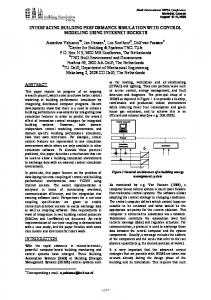
Figure 1: External view of the studied building (3D Google Map) Default Control Strategies The implemented control strategy was a set of predefined rules based on the building control specification2 . The control sequences are summarized as follows: 1. The economizer control was only to maintain the minimum outdoor air mass flow rate of 1.0476 kg/s. 2. A rule-based control was implemented for the temperature set-point reset of the air entering the supply air fan, TESF , as a function of the ambient temperature (See Figure 2 and Figure 3).

Figure 3: Temperature set-point reset for the air entering the supply air fan 3. ON-OFF controls for the boiler and the chiller unit were based on the outdoor air temperature. The

this study, Dymola version 2013 (32-bit) is utilized as the Modelica simulation environment from the technical report, ”Building 101 TRNSYS Baseline Control Logics” written by United Technologies Research Center

2 Obtained

- 3268 -

Proceedings of BS2013: 13th Conference of International Building Performance Simulation Association, Chambéry, France, August 26-28

Figure 2: Schematic of the HVAC system

4.

5.

6.

7.

threshold temperatures were 16.7 o C and 7 o C, respectively. The temperatures of hot water leaving for the boiler and chilled water leaving the cooling coil were assumed to be fixed at 82.1o C and 5o C. It was also assumed that pumps for hot/cold water were turned on and off according to the ON-OFF signals of the boiler/chiller. The mass flow rates of hot and chilled water were adjusted to meet the pre-defined set-point temperature, TESF . It was controlled by a PI controller with 0.07 kg/s-o C for the proportional gain and 3600 seconds for the integral time constant. The control output was in the range [0, 1] where the maximum control signal corresponded to a maximum flow rate of the hot water supply. The supply air mass flow rate for each zone was regulated to maintain a zone air temperature setpoint of 21.11 o C. A PI controller with a propositional gain of 1.5 kg/s-o C and an integral time constant of 3600 seconds was used. The range of the controller output was [0.4, 1] where the 0.4 represented the minimum required ventilation air flow rate with respect to a maximum supply air for each zone. The PI controller manipulated the hot water supply mass flow rate for each VAV box. The control variable was the zone air temperature. The proportional gain and the integral time constant were 0.01 and 3600 s, respectively. The supply air fan was controlled to meet the summation of all supply air flow rates for all zones determined by the VAV air flow rate control.

Model Comparison Envelope Models It is important to explain the differences in the building envelope models between TRNSYS and Modelica. TRNSYS computes the heat transfer through opaque constructions using a conduction transfer method. This results in a finite sum representation which needs

to be evaluated every time base (the default value of one hour Klein et al. (2004)) in order to compute surface temperatures. The window simulation is based on the data sets which contain the spectrally averaged window properties as a function of solar incident angle. The properties are pre-calculated from Window Program (Mitchell et al. (2001)). The treatment of long-wave radiation in default is based on ,so called, star network where long wave radiation exchange between the inside surfaces and the convective heat flux from the inside surfaces to the zone air are linearly approximated. The Modelica building envelop model uses a finite difference scheme to compute the time rate of change of the wall temperatures. This results in a coupled system of linear ordinary differential equations with temperatures as state variables. This equation is integrated with the same time step as the system simulation. The window simulation is a layer-by-layer simulation similar to the Window 6 program. Longwave radiation is based on an approximate view-factor calculation, which we configured to be computed as a linearized equation. Besides the two high fidelity models mentioned above, we also developed a reduced-order model (ROM). The model construction for 20 rooms (9 thermal zones) was based on the formulation described in (Kim and Braun, 2012). To develop the ROM, a finite volume formulation was used to describe the heat conduction through walls. On the external walls an energy balance was applied considering convective heat exchange, as well as short and long wave radiations. The radiosity method was utilized to express the net heat flux under the assumption that the walls were gray, diffuse and opaque. The long-wave interaction terms were linearized and fixed convective heat transfer coefficients were assumed to construct a linear time invariant model for the building thermal network. The final form of the state-space building envelope system is:

- 3269 -

x(t) ˙ = Ax(t) + Bu u(t) + Bw w(t) y(t) = Cx(t)

(1)

Proceedings of BS2013: 13th Conference of International Building Performance Simulation Association, Chambéry, France, August 26-28

where the state variable (x(t) 2 Rn ) contains all temperature nodes in the thermal network, the input (u(t) 2 Rp ) represents mechanical heat addition/removal rate, and the input (w(t) 2 Rq ) represents several exogenous terms, including the heat flow due to solar radiation, outdoor air temperature, long-wave interaction between sky/ground and exterior walls. The output (y(t) 2 Rm ) is chosen to be zone air temperatures. Although (linearly approximated) mean radiant temperature, which is required to evaluate a thermal comfort index such as Predicted Mean Vote (PMV), can be easily included in the output, it is not included in this study because only zone air temperatures are compared. Based on the compact state-space representation in Equation 1, a balanced truncation method (Moore, 1981) was applied to the representation to generate a ROM. The resulting ROM has 74 state dimensions (n) and 65 input channels (p + q). The comparison of simulation results by different multi-zone envelope models are presented in Table 1, where maxMEAN and maxRMS represent the maximum values of mean and root mean square differences of the zone air temperatures over simulation period of a year and over all zones, i.e.

maxM EAN ⌘ max

(

N

1 X ( Ti [k] N

Tj [k])

k=0

8v N