526
IEEE TRANSACTIONS ON CONTROL SYSTEMS TECHNOLOGY, VOL. 14, NO. 3, MAY 2006
Direction-Dependent System Modeling Approaches Exemplified Through an Electronic Nose System Fredrik Rosenqvist, Ai Hui Tan, Keith Godfrey, and Anders Karlström
Abstract—The modeling of processes exhibiting direction-dependent behavior is considered. Depending on the application, different models may be suitable. This brief is concerned with the use of Wiener models and piecewise-linear (PWL) models. These approaches are applied to data from an electronic nose system, for which knowledge of the physical principles is combined with system identification methods. Both models are found to provide close approximations to the behavior of the system itself. Index Terms—Direction-dependent systems, electronic nose systems, identification, modeling, nonlinear systems, perturbation signals, piecewise-linear (PWL) models, pseudorandom sequences, Wiener models.
I. INTRODUCTION
D
IRECTION-DEPENDENT systems have dynamics that are different when the output is increasing from those when the output is decreasing. There are many examples of such behavior in industrial processes given in the literature. These include gas-turbine engines, chemical processes, and nuclear reactors [1]; distillation columns [2]; thermomechanical wood-chip refiners [3]; automotive suspensions [4]; and electronic nose systems [5]. There are several reasons for direction-dependent behavior. For example, in the case of the gas-turbine engine experiments reported by Godfrey and Moore [1], in which the fuel flow was perturbed, it was thought that the engine itself should have a linear response over the small amplitude range of the applied perturbations. It was therefore almost certain that the direction-dependent behavior resulted from the input (fuel flow) transducer being faster in the downward direction than in the upward direction. Turner et al. [2] note that direction-dependent behavior “is a typical feature observed on distillation columns, since it is easier (and therefore faster) to make a 99% product composition less pure than it is to make it more pure.” In automotive suspension systems, direction-dependent behavior can result from nonlinear dampers. In the electronic nose experiments reported by Tan and Godfrey [5], with data from the same system being used in the present brief, the source of this behavior was due to the adsorption of the target gas on the metal–oxide–semiconductor (MOS) sensor surface (dynamics Manuscript received in final form August 17, 2005. Recommended by Associate Editor K. Hunt. F. Rosenqvist is with Solvina AB, SE-421 30 Västra Frölunda, Sweden (e-mail:
[email protected]). A. H. Tan is with the Multimedia University, 63100 Cyberjaya, Malaysia (e-mail:
[email protected]). K. Godfrey is with the University of Warwick, Coventry CV4 7AL, U.K. (e-mail:
[email protected]). A. Karlström is with the Chalmers University of Technology, SE-412 96 Göteborg, Sweden (e-mail:
[email protected]). Digital Object Identifier 10.1109/TCST.2005.860520
in the downward direction) being faster than its desorption (dynamics in the upward direction). In contrast to the number of industrial applications, theoretical results for direction-dependent systems are very limited; to date, they are available for processes with first-order dynamics in both directions, perturbed with either binary signals [4] or ternary signals [6]. Interest has therefore turned to alternative methods of modeling such processes. Three approaches have so far been reported. The first is based on piecewise-linear (PWL) models [7], [8], in which the PWL models switch between two linear time-invariant (LTI) subsystems, with the direction of the input determining the switching. Given this modeling approach, theoretical results are available when it comes to parameter estimation [9] and controllability [10]. In addition, this approach has been applied to data from a thermomechanical wood-chip refiner [3]. The second approach is to use a Wiener model [11], which has been applied to data from simulated systems and from an electronic nose experiment [5], [12]. The third approach has been to use a recurrent neural network approximation using an architecture proposed by Turner et al. [2]; this has also been applied to data from simulated systems and from an electronic nose experiment [5]. In the present brief, the Wiener and PWL modeling approaches are compared with data from the same electronic nose system as in the study conducted by Tan and Godfrey [5]. Both approaches are found to provide close approximations to the behavior of the system itself. In addition, the analysis in this brief describes how direction-dependent processes can be modeled using system identification methods in combination with a discussion of the physical principles in order to confirm that a direction-dependent modeling approach is appropriate. II. FUNDAMENTALS OF ELECTRONIC NOSES There has been significant progress during the past two decades in the area of gas sensor development, particularly in the procedure to identify and quantify attributes of an examined mixture [13]. Such sensors are quite complex and consist normally of a modulator such as selective filters, which changes the gas composition in a controlled way, and a sensor array that gives a signal related to the composition and concentrations of the species in the mixture. Features or parameters are then extracted from the raw signal, producing a signal vector that is examined using a pattern recognition routine to predict or classify some interesting properties of the analyzed gas mixture. One of the most common types of gas sensor, which has been studied for over 20 years, is the electronic nose. The term “electronic nose” was originally coined for an odor measuring system and has been defined as [14] “ an instrument, which comprises an array of electronic chemical sensors with partial
1063-6536/$20.00 © 2006 IEEE
IEEE TRANSACTIONS ON CONTROL SYSTEMS TECHNOLOGY, VOL. 14, NO. 3, MAY 2006
527
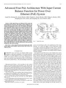
specificity and an appropriate pattern recognition system, capable of recognizing simple or complex odors.” These sensors are often based on MOS field-effect transistor (MOSFET) technology, but several other types of substrates such as metal–oxide sensors, conducting polymer chemo resistors, optical sensors, and oscillation sensors can be classified as electronic noses as well. A significant feature of such sensors is that they are nonlinear and, in simplified cases, can be described as a direction-dependent system [5]. For example, a MOS sensor can be modeled using the adsorption–desorption reaction described by Fig. 1. Structure of the Wiener model with first-order dynamics.
AS
AS
(1)
where AS corresponds to the adsorbed species, represents an empty adsorption site, {AS} represents an occupied site, is the forward rate constant, and is the backward rate constant. Denoting the fractional occupancy of adsorption sites and the concentration of the target gas by and , respectively, gives (2) . The nonlinearity arises from the term The measured output is the voltage across the sensor. The voltage is inversely proportional to the conductance, which is linearly related to . The concentration, in (2), is the input to the process. In the experiment conducted, acetone was used to increase , whereas air was used to decrease . With a binary input perturbation, takes two different values, and the system behaves in two different modes. The dynamics in the upward direction are slower than those in the downward direction due to the fact that the adsorption of acetone on the MOS sensor surface is faster than its desorption. A common problem in gas sensors is a baseline drift [15], [16]. Holmberg et al. [17] considered the gas sensor as a timevarying dynamic system in order to compensate for the drift which worked efficiently in classification problems but has not been studied for problems with continuously varying gas concentrations. In the experiments described in this brief, the drift can be neglected as the total experimentation time has been minimized. In addition, as the mean in the output signal is always removed prior to the parameter estimation process, the effects of drift can be neglected. III. DIRECTION-DEPENDENT MODELING STRATEGIES Nonlinear processes may be modeled in several different ways. General modeling approaches, such as Volterra functional series [18] or neural networks, can be found in the literature. These models are, however, not always easy to comprehend theoretically and physically. If the process is thought to be direction-dependent, model structures designed to cope with this behavior may be applied. These models are simpler in structure, and they allow a better insight into the physical characteristics of the process. The direction-dependent modeling approaches used in this brief are Wiener models [11] and PWL models [7]. The Wiener models are block-oriented and have a structure in
which dynamic LTI subsystems precede instantaneous nonlinearities. The PWL models switch between two LTI subsystems, where the input direction schedules the switching. A. Wiener Models The Wiener model has been shown to generate input–output (I/O) data resembling those of a first-order, continuous-time direction-dependent process in the form [12] (3) where if if
(4)
The input signal is , and the output signal is , corresponds to the continuous time. For the where Wiener model in Fig. 1, the notation is used for the output as this model structure is used as a predictor. The Wiener model consists of a constant path, a linear path, a quadratic path, and a cubic path. In practice, contributions from fourth-order and higher order terms are very small and can be neglected [12]. The quadratic path is added to or subtracted from the total output depending on the dynamics of the direction-dependent process. If the direction-dependent process in (3) has faster dynamics in ), the sign of the quadratic path the increasing direction ( in the Wiener model is set to be negative in order to match (3); otherwise, it is set to be positive. It has been shown that pseudorandom binary signals based on maximum-length sequences are the most suitable signals for the detection of the direction-dependent behavior [4]. When these signals are used to perturb a direction-dependent process, coherent patterns are observed in the input-output cross-correlation function. These are not present when other kinds of pseudorandom binary signals are used. In obtaining the theoretical parameters of the Wiener model, the terms in the I/O cross-correlation function were developed for a first-order process perturbed with a maximum-length binary (MLB) signal and an inverse-repeat MLB signal [12]. The constant term, the linear term, the quadratic term, and the cubic term of the Wiener model can be matched separately using theoretical analysis [12]. A simpler method is to use an optimization algorithm, such as the function fminunc in the MATLAB Optimization Toolbox [19], where the default
528
IEEE TRANSACTIONS ON CONTROL SYSTEMS TECHNOLOGY, VOL. 14, NO. 3, MAY 2006
algorithm is based on least-squares optimization using the Gauss–Newton method. This algorithm was used to match the output of the Wiener model with the output data of the direction-dependent process described in this brief. B. Piecewise-Linear Models PWL modeling of direction-dependent processes has, in previous literature, involved models whose subsystems are LTI and in which the switching is ruled by the sign of the change in the and input signal [9]. If the discretized input signal is the output signal is , the state–space description from to the output change the input change becomes
and is called the delayed-switching model, as the switching is delayed for the higher order parameters, which can be observed by considering how the updates of ’s and ’s depend on the time instants and , respectively. Note that the first-order parameters behave identically for the two models. To estimate the parameters in (8) utilizing the prediction error method (PEM) [22], a predictor is to be derived from the PWL representation. As for LTI models, different types of predictor can be derived depending on where the disturbances are expected to enter the system. The computationally simplest predictor is the piecewise-linear, autoregressive with external input (PWARX) [7] (11)
(5) is the discrete time, is the where is defined as state vector, and the switching function (6) In this PWL extension of the LTI state–space representation, the , , and set of system matrices changes as the input changes signs. The signal values of are computed as the sum of the changes added to the value of at the initial time (7) To estimate a parametric model of a direction-dependent process from I/O data, it is preferable to consider the input and output as in (5). The I/O form of direction-dependent changes processes is commonly represented in terms of PWL dynamics (8) where the inverse shift operator is defined such that . The parameter depends on , as described in (6). However, it is not obvious which determines the active submodel for a given parameter. In the for literature, the common interpretation is that all the parameters in (8) [7], [20], [21]. This form (9) is called the instant-switching model, as all the parameters switch simultaneously, which can be observed by considering . how the updates of the ’s and ’s depend on There is also another form that can be converted into a corresponding state–space form with the structure of (5) [8]. This form is (10)
When using this predictor, the parameter estimation becomes a linear least-squares problem with a drawback that, in the presence of high-frequency disturbances, the estimated model tends to get faster responses than the actual process. The usual way to overcome this problem is to filter the I/O data. One predictor that completely separates the disturbance model from the process model is the piecewise-linear, output-error model (PWOE) [9] (12) However, the computational effort increases in this case. IV. EXPERIMENT ON AN ELECTRONIC NOSE SYSTEM A data set from an electronic nose experiment has been fitted using a Wiener modeling approach and a neural network modeling approach [5]. In the present brief, direction-dependent PWL models have been computed from the same set of I/O to data. Since the transformation in (5) from increases the frequency content of the data, and since the frequency content in the given data is already high, the PWL predictor was modified for this experiment. The switching is still governed by as described in (6), but function the I/O representation in (8) was adjusted to (13) and the predictors in (11) and (12) were adjusted accordingly. Further, a time delay was introduced here. A. Estimation and Validation In order to fit a selected model to a given set of data, there are traditionally different methods to pursue. Six possible objective functions for Wiener models were studied in an earlier work [23], and these are minimizing the following: 1) sum of squares of the error in the cross-correlation functions; 2) sum of the absolute error in the cross-correlation functions; 3) sum of squares of the error in the outputs;
IEEE TRANSACTIONS ON CONTROL SYSTEMS TECHNOLOGY, VOL. 14, NO. 3, MAY 2006
4) sum of the absolute error in the outputs; 5) sum of squares of the error in the frequency response, taking into account both magnitude and phase; 6) sum of the absolute error in the frequency response, taking into account both magnitude and phase. Initial values were specified for each parameter before the start of the optimization procedure, and these were obtained through observation from initial simulations. It was found that the results obtained using different methods are in reasonably close agreement with one another. The parameters of the PWL models were estimated using PEM [22]. This method is based on the minimization of a norm criterion that penalises the error in the outputs. A Gauss–Newton method was used for the optimization, where an LTI estimate was used as initial guess. For the Wiener modeling as well as for the PWL modeling, the optimization objective was to minimize the mean-square error (MSE) of the outputs MSE
(14)
where
(15) For validation, an additional set of input and output data was acquired. The simplest validation test is ocular examination, determining whether the characteristics of the process are captured by the models. Besides comparing the model with the output, the computation of the residuals as a function of time is relevant. This is a good first measure of how well the model agrees with the process, but it should not be completely relied upon. Hence, some quantitative measures were also used. These are the MSE and the mean absolute error (MAE) MAE
(16)
Besides the statistical analysis, it is useful to observe whether the process dynamics are indeed different for the two directions, when a process is suspected to be direction dependent. One way to do this is to study the step responses in both directions so that the differences can be assessed. For the PWL modeling, it should also be evaluated to what extent the parameters separate. B. Results The identification data obtained using an MLB signal are shown in Fig. 2. Direction-dependent models of PWL type were computed from these data for comparison with the Wiener models computed from the same data. For validation, LTI models were also computed. The validation data consist of a set generated from a different MLB signal. All results and comparisons refer to the validation data. Second-order PWL models were significantly better than the first-order ones, and therefore they are the only ones considered here. In order to achieve as good a fit as possible, the time delay must be adjusted. For both the instant-switching PWOE
529
Fig. 2. Identification data with MLB input.
model (PWOE2I) and the delayed-switching PWOE model (PWOE2D), a delay of six samples, corresponding to 6 s, gave the best fit. For the linear output-error model (LTIOE2), a delay of seven and eight samples gave the best fit; the model with , however, gave an almost equally good fit. For the different ARX models, the best fits were in the same neighborhood in terms of delay. The PWARX models, however, consistently gave less accurate fits than their corresponding PWOE models, regardless of the choice of . Consequently, the delay was fixed at six samples, and only the PWOE models were considered. Since the instant and delayed-switching models exhibit very similar properties with these data, only the PWOE2I model was used for comparison. The modeling of electronic nose data using a Wiener model has previously been considered [5], where a delay of three samples in the output, identified from the I/O cross-correlation function, was removed prior to any identification test. In the current brief, a variable delay was introduced when optimizing the Wiener model and the model that resulted in the smallest MSE in the output was selected. It was found that this corresponds to a delay of six samples between the actual data and the Wiener model output. The validation data show that the direction-dependent models give better fits than an LTI one (see Fig. 3). Although the difference is not very clear when studying medium-to-high-frequency data, it can be seen that the direction-dependent models respond more slowly to increasing input and more quickly to decreasing input, in the same way as the measured data. More information is revealed when analyzing the residuals in Fig. 4. It can be concluded that the variation is significantly larger for the LTI model than it is for both the direction-dependent ones. In Table I, the MSEs are shown for both the LTI and the direction-dependent models. Comparing the MSE, the PWL model has the smallest error. While the MSE for the Wiener model is slightly larger than that of the LTI model, this is mainly due to the mismatch in only a few samples in a period. When comparing the MAE, the Wiener model has a better fit than the LTI model. In Table II, it is also shown that the PWL model separates the parameters, which motivates the usage of a direction-dependent model for this process. It should be pointed out that the
530
IEEE TRANSACTIONS ON CONTROL SYSTEMS TECHNOLOGY, VOL. 14, NO. 3, MAY 2006
TABLE II PARAMETERS OF THE OPTIMIZED LTI, PWL, AND WIENER MODELS
Fig. 3. Validation data. The different models y^ (dashed) are compared with the measured output data (solid).
Fig. 5. Unit step-responses of the PWL model (dashed line), the Wiener model (dotted line), and the LTI model (solid line). The negative steps are here plotted as positive for comparison.
good fit, the models that allow different dynamics for different input and output directions resulted in more accurate fits. V. DISCUSSION
Fig. 4. Residuals obtained for the different models.
TABLE I ERROR MEASUREMENTS USING LTI, PWL, AND WIENER MODELS
optimization of the Wiener parameters could be improved by using an inverse-repeat MLB signal as input [5]. In order to evaluate how well the direction-dependent models separate the increasing and decreasing dynamics, their unit step-responses are depicted in Fig. 5. The separation in speed and gain is clear. It can also be concluded that the LTI model achieved a reasonable compromise given these data. The physical description in combination with the statistical models illustrates that direction-dependent descriptions are appropriate for electronic nose processes. From the technical description in (1) and (2), it is clear that the process shows different dynamics depending on whether the net reaction is adsorption or desorption. Even though the LTI model provided a reasonably
The electronic nose application in the previous section illustrates that there are processes in which a direction-dependent model description is suitable. This could be considered as the sensor part in a more general industrial process. Depending on the application, different direction-dependent descriptions may be suitable. The Wiener approach is one good technique for modeling direction-dependent processes; an important advantage of such a model, besides its simplicity due to its block-oriented structure, is that it does not exhibit any switch. If this process were to be used in an online self-tuning control system [24], there is an advantage not to have a switch in the model structure as the input signal to the switching function could be corrupted by noise. The PWL direction-dependent model, on the other hand, has an inherent switch. This approach is another good technique and could be useful in the case where the control system is able to deal with a switching model. In such a case, the PWL model has an advantage that the switching is able to capture an infinite order of nonlinearity. The LTI model could be considered acceptable, but not ideal when it comes to designing a control system; in this case, the two subsystems from the PWL model could be used for validation of a robust controller. REFERENCES [1] K. R. Godfrey and D. J. Moore, “Identification of processes having direction-dependent responses, with gas-turbine engine applications,” Automatica, vol. 10, no. 10, pp. 469–481, 1974.
IEEE TRANSACTIONS ON CONTROL SYSTEMS TECHNOLOGY, VOL. 14, NO. 3, MAY 2006
[2] P. Turner, G. Montague, and J. Morris, “Nonlinear and direction-dependent dynamic process modeling using neural networks,” Proc. Inst. Elect. Eng.—Control Theory Appl., vol. 143, no. 1, pp. 44–48, 1996. [3] F. Rosenqvist and A. Karlström, “Direction-dependent responses to the hydraulic pressure in TMP processes,” in Proc. Control Systems Conf., Quebec, QC, Canada, Jun. 2004, pp. 113–120. [4] A. H. Tan and K. R. Godfrey, “Identification of processes with directiondependent dynamics,” Proc. Inst. Elect. Eng.—Control Theory Appl., vol. 148, no. 5, pp. 362–369, 2001. [5] , “Modeling of direction-dependent processes using Wiener models and neural networks with nonlinear output error structure,” IEEE Trans. Instrum. Meas., vol. 53, no. 3, pp. 744–753, 2004. [6] A. H. Tan, “Identification of direction-dependent processes using maximum length ternary signals,” Proc. Inst. Elect. Eng.—Control Theory Appl., vol. 150, no. 2, pp. 170–178, 2003. [7] J. Roll, A. Bemporad, and L. Ljung, “Identification of piecewise affine systems via mixed-integer programming,” Automatica, vol. 40, no. 1, pp. 37–50, 2004. [8] F. Rosenqvist and A. Karlström, “Realization and estimation of piecewise-linear output-error models,” Automatica, vol. 41, no. 3, pp. 545–551, 2005. , “Piecewise-linear output-error methods for parameter estimation [9] in direction-dependent processes,” in Hybrid Systems: Computation and Control. ser. Lecture Notes in Computer Science, R. Alur and G. J. Pappas, Eds. New York: Springer-Verlag, 2004, vol. 2993, pp. 493–507. , “Controllability of direction-dependent processes,” in Proc. Conf. [10] Decision Control, vol. 4, Maui, HI, Dec. 2003, pp. 3384–3389. [11] S. Billings and S. Y. Fakhouri, “Identification of nonlinear systems using the Wiener model,” Electron. Lett., vol. 13, no. 17, pp. 502–504, 1977. [12] H. A. Barker, A. H. Tan, and K. R. Godfrey, “Wiener models of directiondependent dynamic systems,” Automatica, vol. 39, no. 1, pp. 127–133, 2003.
531
[13] J. W. Gardner and P. N. Bartlett, Electronic Noses—Principles and Applications. Oxford, U.K.: Oxford Univ. Press, 1999. [14] , “A brief history of electronic noses,” Sens. Actuators B, vol. 18, no. 1–3, pp. 210–211, 1994. [15] T. Eklöv, “Methods to improve the selectivity of gas sensor systems,” Ph.D. dissertation, Lindköping Univ., Linköping, Sweden, 1999. [16] M. Fryder, M. Holmberg, F. Winquist, and I. Lundström, “A calibration technique for an electronic nose,” in Proc. Int. Conf. Solid-State Sensors Actuators Eurosensors, 1995, pp. 683–686. [17] M. Holmberg, F. Davide, C. Di Natale, A. D’Amico, F. Winquist, and I. Lundström, “Drift counteraction in odour recognition applications: Lifelong calibration method,” Sens. Actuators B, vol. 42, pp. 185–194, 1997. [18] V. Volterra, Theory of Functionals and of Integral and Integrodifferential Equations. London, U.K.: Blackie, 1930. [19] T. Coleman, M. A. Branch, and A. Grace, Optimization Toolbox for Use With MATLAB. Natick, MA, USA: The Mathworks, Inc., 1999. [20] S. Billings and W. Voon, “Piecewise linear identification of nonlinear systems,” Int. J. Control, vol. 46, pp. 215–235, 1987. [21] G. Ferrari-Trecate, M. Muselli, D. Liberati, and M. Morari, “Identification of piecewise affine and hybrid systems,” in Proc. Amer. Control Conf., Arlington, VA, Jun. 2001, pp. 3521–3526. [22] L. Ljung, System Identification—Theory for the User. Englewood Cliffs, NJ: Prentice-Hall, 1999. [23] A. H. Tan, “System identification and its applications, with emphasis on direction-dependent processes,” Ph.D. dissertation, School of Eng., Univ. of Warwick, Coventry, U.K., 2002. [24] A. Dunoyer, L. Balmer, K. J. Burnham, and D. J. G. James, “On the discretization of single-input single-output bilinear systems,” Int. J. Control, vol. 68, no. 2, pp. 361–372, 1997.