Compensating for Missing Data from Longitudinal Studies Using ...

JSS

Journal of Statistical Software June 2007, Volume 19, Issue 7.

http://www.jstatsoft.org/

Compensating for Missing Data from Longitudinal Studies Using WinBUGS Gretchen Carrigan

Adrian G. Barnett

University of Queensland

University of Queensland

Annette J. Dobson

Gita Mishra

University of Queensland

University of Queensland

Abstract Missing data is a common problem in survey based research. There are many packages that compensate for missing data but few can easily compensate for missing longitudinal data. WinBUGS compensates for missing data using multiple imputation, and is able to incorporate longitudinal structure using random effects. We demonstrate the superiority of longitudinal imputation over cross-sectional imputation using WinBUGS. We use example data from the Australian Longitudinal Study on Women’s Health. We give a SAS macro that uses WinBUGS to analyze longitudinal models with missing covariate date, and demonstrate its use in a longitudinal study of terminal cancer patients and their carers.

Keywords: missing data, multiple imputation, longitudinal data, WinBUGS, SAS.

1. Introduction Missing data is a common problem in survey-based research. Ignoring any missing data by using a complete case analysis can produce biased results. Biases occur when participants with complete data are systematically different from those with missing data. Longitudinal studies are especially susceptible to such bias, as missing data accumulates over time due to wave non-response and participant drop-out. One method of compensating for missing data is imputation. Over the past twenty years the body of literature on imputation theory and methodology has grown considerably and software has evolved accordingly. However, there has been relatively little work on imputation in a longitudinal setting. There are several theoretical approaches to imputation. Raghunathan (2004) reviews such

2

Compensating for Missing Longitudinal Data Using WinBUGS

approaches and identifies three classes: weighted estimating equations, multiple imputation, and likelihood-based formulations. Ibrahim et al. (2005) identify fully Bayesian as a fourth class. Weighted estimating equations (WEE) weight records with complete data to compensate for similar cases with missing data. Most recently, literature has focussed on improving estimates of variance (Robins et al. 1994, 1995) as WEE, when unadjusted, underestimate the true variance in the data. Implementation of WEE currently relies on model-specific, user-defined algorithms, rather than standard procedures in mainstream statistical packages. Multiple imputation (MI) uses Bayesian simulation to fill in missing data, drawing together results from repeatedly imputed datasets. See Rubin (1987) for a comprehensive coverage of multiple imputation. Fully Bayesian (FB) models extend MI methodology by jointly simulating the distributions of variables with missing data as well as unknown parameters in a regression equation. In FB the analysis and imputation models are fully and simultaneously specified. Maximum likelihood (ML) techniques also rely on fully specified models, but differ from FB in that parameter estimates are constructed using likelihood-based approximations, rather than Bayesian simulation. Maximum likelihood approaches to imputation are often intractable in mainstream software packages. Implementation relies upon strict assumptions about patterns of missingness that are frequently violated in complex survey data. While MI procedures exist in a range of software packages such as SAS (SAS Institute Inc. 2003), Stata (StataCorp. 2003), S-PLUS (Insightful Corp. 2003), and R (R Development Core Team 2007), they generally rely on the assumption that data are multivariate normal or can be approximated by a multivariate normal distribution (Schafer 1997). More recent work on chained regression equations has led to a number of add-on packages that can incorporate categorical data: MICE in SPLUS (van Buuren and Oudshoorn 1999), Ice in Stata (Royston 2005), and IVEware for SAS (Raghunathan et al. 2002). However, the authors have still had difficulty in incorporating longitudinal information into the imputation methodology of these programs. FB techniques are most suited to longitudinal imputation, as they can incorporate hierarchical structure into the modelling process, and, like chained regressions, they have the capability to systematically deal with categorical data. The software packages WinBUGS (Spiegelhalter et al. 2003) and MLwiN (Rasbash et al. 2005) both use a FB framework. Cowles (2004) and Woodworth (2004) both provide a useful overview to WinBUGS, while Carpenter and Kenward (2005) and Congdon (2001) present introductory examples of FB imputation with missing data. Pettitt et al. (2006) and Qiu et al. (2002) present thorough analyses in the context of missing categorical data. The aim of this paper is to demonstrate WinBUGS’s capacity to compensate for missing longitudinal data, with a particular focus on missing covariate data. We do this by looking at a longitudinal analysis of diabetes incidence in Australian women. In Section 2 we introduce the motivating example from the Australian Longitudinal Study on Women’s Health. In Section 3 we specify a fully Bayesian model for the incidence of diabetes without and with missing covariate data. In Section 4 we describe its implementation in WinBUGS, and present the results in Section 5. In Section 6 we give a general SAS macro (that calls WinBUGS) for analysing longitudinal models with missing covariate data. We conclude with a discussion and some recommendations in Section 7.

Journal of Statistical Software

3

2. Motivating example Women who are overweight have an increased risk of developing diabetes. However the relative impact of longer-term adiposity and short-term weight changes on the incidence of diabetes is of scientific interest (Mishra et al. 2007). The Australian Longitudinal Study on Women’s Health (ALSWH) is designed to answer such questions as it tracks over time the health and well-being of a representative sample of Australian women (Lee, Dobson, Brown, Bryson, Byles, Warner-Smith, and Young 2005). The ALSWH study collects self-reported data from mail-out surveys every two to three years. For this analysis we used data from the mid-aged cohort of women who were aged 45 to 50 at the time of the initial survey in 1996 (S1). Subsequent surveys occurred in 1998 (S2), 2001 (S3), and 2004 (S4). At S1 13,716 women agreed to take part in the longitudinal study and by S4 10,905 women remained. Key variables for the analysis of diabetes incidence and weight are outlined below. At S1 women were asked if they had ever been diagnosed with diabetes. At S2, S3 and S4 women were asked if they had been diagnosed with diabetes since the previous survey. Using this data women were classified into one of the following groups: existing case at S1, incident case between S1 and S2, incident case between S2 and S3, incident case between S3 and S4, free from diabetes, or unknown. Women were asked to report their height and weight at each survey. Self-reported heights from the first three surveys were used to obtain a single estimated value for each woman by averaging the available data. Body mass index (BMI) for each woman at S1 was calculated as self-reported weight (kilograms) at S1 divided by the square of estimated height (metres). BMI was categorized as (according to the World Health Organization (2000)): ‘underweight’, < 18.5 kg/m2 ; ‘healthy weight’, [18.5, 25) kg/m2 ; ‘overweight’, [25, 30) kg/m2 ; ‘obese’, [30, 35) kg/m2 ; or ‘very obese’, ≥ 35 kg/m2 . Fewer than 2% of women were classified as ‘underweight’ at S1, so this category was combined with the ‘healthy weight’ group. At S1 women were asked what they would like to weigh. Responses were categorized into: happy/like to weigh more, like to weigh 0 to 5 kg less, like to weigh 5 to 10 kg less, like to weigh more than 10 kg less.

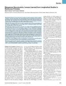
3. Model specification Examining the association between health and weight is often difficult in survey data because weight is a sensitive question and is sometimes not reported. For example, in the ALSWH at S1 545 women (4.0%) did not report their weight, whereas for the other variables used in this paper the average percent of missing was 1.3%. If women who are overweight are less likely to report their weight then a complete case analysis could well underestimate the true association between weight and diabetes incidence. Figure 1 gives a graphical summary of our model. The model is split into the imputation and diabetes components. In the diabetes component we examined the association between BMI at S1 and annual percentage weight change on the incidence of diabetes, adjusting for age at baseline. BMI at S1 represented longer-term adiposity while annual percentage weight change represented short-term weight change. Because we were interested in weight change before diabetes onset, weight change was measured in the survey period prior to reported incidence

4

Compensating for Missing Longitudinal Data Using WinBUGS

Figure 1: Model of the association between diabetes incidence and long-term BMI and shortterm changes in weight

(to avoid the risk of ‘reverse causation’ whereby women who were diagnosed with diabetes subsequently lost weight). Therefore, the study population for the analysis was confined to those women who became an incident case between S2 and S3 or S3 and S4, or those who were free from diabetes. Women who became an incident case between S2 and S3 were excluded from the analysis in the following period as they were no longer in the population at risk. As shown in Figure 1 there were different amounts of missing covariates, with likely different reasons for why they were not completed. Rubin defines three potential patterns of missingness: missing completely at random (MCAR), in which there is no systematic difference between the characteristics of those with and without missing data; missing at random (MAR), in which there is a systematic difference but this can be explained by other observed data; and missing not at random (MNAR) where the difference cannot be explained by observed data. We relied on the MAR assumption to build an imputation component into the model using the question, “How much would you like to weigh?” There were far fewer missing responses to the ‘like to weigh’ question compared with actual weight. Also, the ‘like to weigh’ variable at S1 was highly correlated with self-reported weight at all surveys (Mishra and Dobson 2004). Hence we used ‘like to weigh’ to impute missing weights at each survey. For each imputed weight we recalculated BMI at S1 and percentage weight change. Women for whom height was unknown (3.2%) or who didn’t respond to the ‘like to weigh’ question (3.2%) were excluded from the analysis. For illustrative purposes we constructed three separate models:

Journal of Statistical Software

5

(i) A complete case model (7113 women), (ii) A cross-sectional imputation model (9557 women), (iii) A longitudinal imputation model using random effects to incorporate within-subject correlation (9557 women). Models (ii) and (iii) both had the diabetes and imputation component (Figure 1). Model (i) only had the diabetes component. We now describe the three models in more detail.

3.1. Complete case model Let Yit be a binary variable denoting incidence of diabetes for individual i (i = 1, . . . , 7113) at time t (t = 1, 2). The complete case model is then, Yit ∼ Bernoulli(pit ), logit(pit ) = αt + XiT β + Zi(t−1) Ψ where X is a matrix of the time-invariant covariates (BMI at S1, age at S1), Z is a vector containing the single time varying covariate (percentage weight change in the survey period prior to reported incidence) and α is an intercept that varies according to survey (time).

3.2. Cross-sectional imputation model The diabetes component of this model followed the same structure as the complete case model. In the imputation component of the model, we assumed that the weight of individual i (i = 1, . . . , 9557) at survey s (s = 1, . . . , 4) was distributed as: Wis ∼ Normal(µis , σ 2 ), µis = γ + ϕt + LTi φ, where L is a vector containing the response of each individual i to the ‘like to weigh’ question. Thus weight for individual i at survey s was described by a population mean γ plus an increment of ϕ at each survey, and was adjusted according to the response of individual i to ‘like to weigh’ at S1 (φ). The estimates of γ, ϕ and φ were based on records with partial or complete data. Women with a missing weight (Wis ) had their weight imputed from a Normal distribution with mean µ ˆis and variance σ ˆ2. Note that the diabetes component is evaluated over two time periods (t = 1, 2, surveys 3 and 4) whereas the weight component is evaluated over four time periods (s = 1, 2, 3, 4, surveys 1 to 4). This meant that we used the maximum amount of information to impute weight, whilst excluding surveys 1 and 2 from the diabetes component because we were only interested in incident cases.

3.3. Longitudinal imputation model The diabetes component of the model followed the same structure as the complete case model. We introduced a random intercept into the imputation component of the model to incorporate

6

Compensating for Missing Longitudinal Data Using WinBUGS

within-subject correlation in weight, and hence take account of the longitudinal study design. The imputation component for weight was: Wis ∼ Normal(µis , σb2 ), µis = γi + ϕt + LTi φ, 2 γi ∼ Normal(λ, σw ).

Instead of a population mean for weight, each subject had her own estimate (γi , known as a random intercept). The total variance in weight from the previous model (σ 2 ) has been 2 , and the between-subject variance σ 2 . The partitioned into the within-subject variance σw b 2 2 ). within-subject correlation is given by ρ = σb /(σb2 + σw

3.4. Inference using Gibbs sampling The models that we have presented above use two parametric distributions (Bernoulli and Normal), with many parameters at several hierarchical levels. An analytical solution to the model is therefore intractable. Fortunately we can make inference about the parameters using Gibbs sampling (the default method in WinBUGS). In Gibbs sampling each unknown parameter is estimated conditional on all the other observed data and the other estimated parameters (for a detailed description of Gibbs sampling see Gelman et al. (2004)). For example, in the hierarchical imputation model, a missing weight would be sampled from a normal distribution with mean µ ˆis and variance σ ˆ 2 . A complete iteration occurs when all the parameters and missing data have been estimated. The next iteration is then based on these estimates and the data. To start the iterations an initial set of values for each unknown parameter and observation is specified. Many iterations are run (usually greater than 1000) in an attempt to converge to a solution. We discuss some of the practical issues of running such iterations in the next section.

4. WinBUGS code To run an analysis in WinBUGS there are four basic requirements: specify a model; load the data; specify initial values; and run the Gibbs sampler. This process is most efficient when the above information is stored in four batch files: an input data file; a file containing the model specification; an initial values file; and a script file that executes WinBUGS commands. We focus here on the model specification file, illustrating the conversion of our three models into a WinBUGS format. Model specification in WinBUGS differs from other standard statistical packages in that the model must be fully and explicitly specified by the user, rather than inserting model specifications into pre-programmed statistical procedures. Information on the construction of the remaining batch files is in Appendix A.

4.1. Complete case model The first lines of code are: model{ for (i in 1:7311){ for (t in 1:nsurvey[i]){

Journal of Statistical Software

7

The model statement opens the model specification file. We looped through records for 7311 individuals at two time points, except where a woman first reported diagnosis of diabetes at S3, in which case she was no longer included in the population at risk at S3 and data from a single time point was used. This condition was achieved through the use of the indicator variable, nsurvey, which took the value of 1 when diabetes incidence occurred between S2 and S3, and took the value of 2 otherwise. In this model t = 1 refers to diabetes incidence between S2 and S3 and weight change between S1 and S2. Similarly t = 2 refers to diabetes incidence between S3 and S4 and weight change between S2 and S3. BMI and age at S1 did not change over time. We specified the distribution of diabetes incidence (diab) to be Bernoulli, diab[i,t] ~ dbern(diab.prob[i,t]); Ending statements with a semi-colon is optional in WinBUGS. Our interest lay in the parameter diab.prob, which represents the probability of becoming an incident case of diabetes. We modelled the relationship between the probability of diabetes and other explanatory variables as follows. logit(diab.prob[i,t])