Compilation of Constraint Systems to Parallel Procedural ... - CiteSeerX

Compilation of Constraint Systems to Parallel Procedural Programs by

Ajita John, B.Sc., B.E., M.S.

Dissertation Presented to the Faculty of the Graduate School of The University of Texas at Austin in Partial Ful llment of the Requirements for the Degree of

Doctor of Philosophy

The University of Texas at Austin December 1997

Compilation of Constraint Systems to Parallel Procedural Programs Publication No. Ajita John, Ph.D. The University of Texas at Austin, 1997 Supervisor: J. C. Browne

An attractive approach to specifying programs is to represent a computation as a set of constraints upon the state variables that de ne the solution and to choose an appropriate subset of the state variables as the input set. But, there has been little success in attaining ecient execution of parallel programs derived from constraint representations. There are, however, both motivations for continuing research in this direction and reasons for optimism concerning success. Constraint systems have attractive properties for compilation to parallel computation structures. A constraint system gives a control ow-free and data ow-free speci cation of a computation, thereby oering the compiler freedom of choice in deriving control structures. All types of parallelism (AND, OR, task, data) can be derived. Either eective or complete programs can be derived from constraint systems on demand. Programs for dierent computations can be derived from the same constraint speci cation through dierent choices of the input set of variables. ii

This dissertation reports on the compilation of constraint systems into task level parallel programs in a procedural language. This is the only research, of which we are aware, which attempts to generate ecient parallel programs for numerical computations from constraint systems. Computations are expressed as constraint systems. A dependence graph is derived from the constraint system and a set of input variables. The dependence graph, which exploits the parallelism in the constraints, is mapped to the target language CODE, which represents parallel computation structures as generalized dependence graphs. Finally, parallel C programs are generated. To extract parallel programs of appropriate granularity, the following features have been included. (i) modularity, (ii) operations over structured types as primitives, (iii) de nition of atomic functions. A prototype compiler has been implemented. The execution environment or software architecture is speci ed separately from the constraint system. The domain of matrix computations has been targeted for applications. Performance results for example programs are very encouraging. The feasibility of extracting ecient and portable parallel programs from domain-speci c constraint systems has been established.

iii

Contents Abstract

v

List of Figures

xii

Chapter 1 Introduction

1.1 Problem Statement and Approach . . . . . . . . . . . . . . . . . . . 1.2 Constraint Systems as Representations of Computations for Parallel Execution . . . . . . . . . . . . . . . . . . . . . . . . . . . . . . . . .

Chapter 2 Background: Constraints

2.1 De nitions . . . . . . . . . . . . . . . . . . . 2.2 Constraint Types . . . . . . . . . . . . . . . 2.2.1 Linear and Non-linear Constraints . 2.2.2 One-way and Multi-way Constraints 2.2.3 Hierarchical Constraints . . . . . . . 2.2.4 Higher-Order Constraints . . . . . . 2.2.5 Meta-Constraints . . . . . . . . . . . 2.2.6 Temporal Constraints . . . . . . . . 2.3 Constraint Graphs . . . . . . . . . . . . . . 2.4 Constraint Satisfaction Techniques . . . . . 2.4.1 Local Propagation . . . . . . . . . . iv

. . . . . . . . . . .

. . . . . . . . . . .

. . . . . . . . . . .

. . . . . . . . . . .

. . . . . . . . . . .

. . . . . . . . . . .

. . . . . . . . . . .

. . . . . . . . . . .

. . . . . . . . . . .

. . . . . . . . . . .

. . . . . . . . . . .

. . . . . . . . . . .

. . . . . . . . . . .

. . . . . . . . . . .

1 1

2

6

8 9 9 9 10 10 10 11 11 12 12

2.4.2 Relaxation . . . . . . . . . . . . . . . . . . . . . . . . . . 2.4.3 Propagating Degrees of Freedom . . . . . . . . . . . . . . 2.4.4 Graph Transformation . . . . . . . . . . . . . . . . . . . . 2.4.5 Miscellaneous Techniques . . . . . . . . . . . . . . . . . . 2.5 Our Approach . . . . . . . . . . . . . . . . . . . . . . . . . . . . . 2.5.1 Types of Constraints Resolved through Our System . . . 2.6 Constraint Systems as Representations of Parallel Computations 2.6.1 Conformance to Desired Property Set . . . . . . . . . . . 2.6.2 The Role of the Type System . . . . . . . . . . . . . . . . 2.6.3 Modular Structure . . . . . . . . . . . . . . . . . . . . . .

Chapter 3 The Constraint Language 3.1 3.2 3.3 3.4 3.5

Type System . . . . . . . . . . . . . . . . . . . . . . . . . . Expressions . . . . . . . . . . . . . . . . . . . . . . . . . . . Constraints . . . . . . . . . . . . . . . . . . . . . . . . . . . Program Structure . . . . . . . . . . . . . . . . . . . . . . . Sample Programs . . . . . . . . . . . . . . . . . . . . . . . . 3.5.1 The Quadratic Equation Solver . . . . . . . . . . . . 3.5.2 The Block Triangular Solver(BTS) . . . . . . . . . . 3.5.3 The Block Odd-Even Reduction Algorithm(BOER) . 3.5.4 The Laplace Equation . . . . . . . . . . . . . . . . .

Chapter 4 The Basic Compilation Algorithm

. . . . . . . . .

. . . . . . . . .

4.1 Phase 1: Generation of Constraint Graphs . . . . . . . . . . . . 4.2 Phase 2: Translation of Constraint Graphs to Directed Graphs 4.3 Phase 3: Generation of Dependence Graphs . . . . . . . . . . . 4.3.1 Resolution of Simple Constraints . . . . . . . . . . . . . 4.3.2 Resolution of Indexed Sets . . . . . . . . . . . . . . . . . v

. . . . . . . . . . . . . .

. . . . . . . . . . . . . . . . . . . . . . . .

. . . . . . . . . . . . . . . . . . . . . . . .

13 13 14 15 15 18 19 19 20 21

22 22 24 24 27 27 28 29 30 34

36 37 40 43 45 46

4.3.3 Resolution of Constraint Module Calls . . . . . . . . . . . . . 4.3.4 The Quadratic Equation Solver through Phase 3 . . . . . . . 4.3.5 Single Assignment Variable Programs . . . . . . . . . . . . . 4.3.6 Generation of either Eective or Complete Programs . . . . . 4.3.7 Extraction of parallelism . . . . . . . . . . . . . . . . . . . . . 4.3.8 Unresolved Constraints . . . . . . . . . . . . . . . . . . . . . 4.4 Phases 4 and 5: Speci cation of Execution Environment and Mapping to Code . . . . . . . . . . . . . . . . . . . . . . . . . . . . . . . . . . 4.5 Procedural Parallel Programs for the BTS and BOER Systems . . . 4.5.1 The BTS System . . . . . . . . . . . . . . . . . . . . . . . . . 4.5.2 The BOER System . . . . . . . . . . . . . . . . . . . . . . . .

50 52 54 55 55 59 63 63 64 65

Chapter 5 Iterative Solutions for Constraint Systems with Cycles 70 5.1 Selection of Term to be Computed . . . . . . . . . . . . . 5.1.1 Unresolved Simple Constraints . . . . . . . . . . . 5.1.2 Unresolved Constraint Module Calls . . . . . . . . 5.1.3 Unresolved Indexed Sets . . . . . . . . . . . . . . . 5.2 Mapping single assignment variables to mutable variables 5.3 Relaxation Methods . . . . . . . . . . . . . . . . . . . . . 5.4 The Laplace Equation Example . . . . . . . . . . . . . . . 5.4.1 The Dependence Graph for the Laplace Equation .

Chapter 6 Execution Environment Speci cation 6.1 6.2 6.3 6.4 6.5

Shared Variables . . . . . . . . . . . . . . . . . Number of Available Processors . . . . . . . . . Data Partitioning with Overlap Sections . . . . Option of not Parallelizing a Module . . . . . . Selecting Operations to be Executed in Parallel vi

. . . . .

. . . . .

. . . . .

. . . . .

. . . . .

. . . . .

. . . . . . . .

. . . . .

. . . . . . . .

. . . . .

. . . . . . . .

. . . . .

. . . . . . . .

. . . . .

. . . . . . . .

. . . . .

. . . . . . . .

. . . . .

73 73 73 75 77 78 79 79

83 84 85 85 86 87

6.6 Choices among Parallel Algorithms to execute some of the Operations 87

Chapter 7 Performance Results

89

Chapter 8 Related Work

97

7.0.1 The Block Triangular Solver (BTS) . . . . . . . . . . . . . . . 89 7.0.2 The Block Odd-Even Reduction Algorithm(BOER) . . . . . . 92 7.0.3 The Laplace Equation . . . . . . . . . . . . . . . . . . . . . . 93

8.1 Constraint Programming . . . . . . . . . . . . . . . . . . . . . . . . . 8.1.1 Consul . . . . . . . . . . . . . . . . . . . . . . . . . . . . . . . 8.1.2 Thinglab . . . . . . . . . . . . . . . . . . . . . . . . . . . . . 8.1.3 Kaleidoscope . . . . . . . . . . . . . . . . . . . . . . . . . . . 8.1.4 Concurrent Constraint Programming . . . . . . . . . . . . . . 8.2 Parallel Programming . . . . . . . . . . . . . . . . . . . . . . . . . . 8.2.1 Automatic Parallelization of Sequential Programs . . . . . . . 8.2.2 Extension of Procedural Languages with Directives for Parallelism . . . . . . . . . . . . . . . . . . . . . . . . . . . . . . . 8.2.3 Parallel Logic Programming . . . . . . . . . . . . . . . . . . . 8.2.4 Parallel Functional Programming . . . . . . . . . . . . . . . . 8.2.5 Equational Systems . . . . . . . . . . . . . . . . . . . . . . . 8.2.6 Miscellaneous Systems . . . . . . . . . . . . . . . . . . . . . .

98 98 98 98 99 99 99

100 100 100 101 101

Chapter 9 Conclusions

103

Chapter 10 Future Work

105

9.1 Contributions . . . . . . . . . . . . . . . . . . . . . . . . . . . . . . . 104

10.1 Extraction of Algorithms . . . . . . . . . . . . . . . . . . . . . . . . 105 10.2 Writing \Good" Speci cations . . . . . . . . . . . . . . . . . . . . . 106 10.3 Choosing a Path in Eective Programs . . . . . . . . . . . . . . . . . 106 vii

10.4 Exploring New Application Areas . . . . . . . . . . . . . . . . . . . . 106 10.5 Extensions to Current Work . . . . . . . . . . . . . . . . . . . . . . . 107

Appendix A CODE A.1 A.2 A.3 A.4 A.5

Nodes . . . . . . . . . . . . . . . . . Arcs . . . . . . . . . . . . . . . . . . Firing rules and Routing rules . . . . Formal speci cation of CODE model A CODE Implementation Overview

Bibliography

. . . . .

. . . . .

. . . . .

. . . . .

. . . . .

. . . . .

. . . . .

. . . . .

. . . . .

. . . . .

. . . . .

. . . . .

. . . . .

. . . . .

. . . . .

. . . . .

. . . . .

. . . . .

108 108 109 110 111 113

117

viii

List of Figures 2.1 Constraint Graph for Temperature Conversion Program . . . . . . . 2.2 Computing the Fahrenheit value of 30 degrees Celsius using Local Propagation . . . . . . . . . . . . . . . . . . . . . . . . . . . . . . . . 2.3 Computing the Celsius value of 100 degrees Fahrenheit using Local Propagation . . . . . . . . . . . . . . . . . . . . . . . . . . . . . . . . 2.4 (a) Cycle in a Constraint Graph (b) Using a Rewrite Rule to break the Cycle . . . . . . . . . . . . . . . . . . . . . . . . . . . . . . . . . 2.5 A Simple Dependence Graph . . . . . . . . . . . . . . . . . . . . . .

14 16

3.1 3.2 3.3 3.4 3.5 3.6 3.7 3.8 3.9 3.10

23 28 29 29 30 30 32 33 34 35

The Type System Layout . . . . . . . . . . . . . . . . . . . . . . . . Constraint Speci cation for the Quadratic Equation Solver . . . . . BTS: Partitioned Lower Triangular Matrix A, Vectors X and B . . . Constraint Speci cation for the BTS System . . . . . . . . . . . . . BTS: Partitioned Lower Triangular Matrix A . . . . . . . . . . . . . Alternate Notation for the Constraint Speci cation for the BTS System Parallel Algorithm for the Cyclic Block Tridiagonal System . . . . . Constraint Speci cation for the BOER System . . . . . . . . . . . . The Laplace Equation Grid . . . . . . . . . . . . . . . . . . . . . . . Constraint Speci cation for the Laplace Equation System . . . . . . ix

11 12 13

4.1 4.2 4.3 4.4 4.5 4.6 4.7 4.8 4.9 4.10 4.11 4.12 4.13 4.14 4.15 4.16 4.17 4.18 4.19 4.20 4.21 4.22 4.23

Constraint Speci cation for the Quadratic Equation Solver . . . . . Constraint Graphs for (a) Rule 1 (b),(c) Rule 2 . . . . . . . . . . . . Constraint Graphs for (a) Rule 3 (b) Rule 4 . . . . . . . . . . . . . . Constraint Graphs for the Quadratic Equation Solver . . . . . . . . Phase 2 for four base cases . . . . . . . . . . . . . . . . . . . . . . . Trees from Phase 2 for the Quadratic Equation Solver . . . . . . . . Generalized Dependence Graph Node . . . . . . . . . . . . . . . . . Indexed Set at a Node in a Tree from Phase 2 . . . . . . . . . . . . . Generated Dependence Graph for an AND Indexed Set . . . . . . . Generated Dependence Graph for an OR Indexed Set . . . . . . . . Dependence Graphs for a Constraint Module Call . . . . . . . . . . . Dependence Graphs for the Quadratic Equation Solver with I = fa, b, cg . . . . . . . . . . . . . . . . . . . . . . . . . . . . . . . . . . . . Dependence Graphs for the Quadratic Equation Solver with I = fa, b, r1g . . . . . . . . . . . . . . . . . . . . . . . . . . . . . . . . . . . Constraint Speci cation for a Simple Example . . . . . . . . . . . . . Dependence Graph showing AND-OR Parallelism . . . . . . . . . . . (a) Parallel Execution of Loop (b) Sequential Execution of Loop . . Generalized Compiled Loop Structure . . . . . . . . . . . . . . . . . Deletion of a Path with Unresolved Constraints . . . . . . . . . . . . Control Flow for the Constraint Compiler . . . . . . . . . . . . . . . Constraint Speci cation for the BTS System with Computed Terms in bold . . . . . . . . . . . . . . . . . . . . . . . . . . . . . . . . . . . Dependence Graph for the BTS Program . . . . . . . . . . . . . . . Constraint Speci cation of the BOER System with Computed Terms in bold . . . . . . . . . . . . . . . . . . . . . . . . . . . . . . . . . . . Dependence Graph for the BOER Program . . . . . . . . . . . . . . x

37 38 39 39 40 43 44 47 48 50 52 53 53 56 57 58 59 62 64 65 66 68 69

5.1 5.2 5.3 5.4 5.5 5.6 5.7 5.8 5.9 5.10

Constraint Speci cation and Input Set with a Cyclic Dependency . Tree from Phase 2 for Constraint Speci cation in Figure 5.1 . . . . A Constraint Graph with a Cycle . . . . . . . . . . . . . . . . . . . An Unresolved Constraint Module Call . . . . . . . . . . . . . . . . Example of an Unresolved Constraint Speci cation . . . . . . . . . Regions of Access by Terms in Figure 5.5 . . . . . . . . . . . . . . Jacobi Relaxation for the Laplace Equation . . . . . . . . . . . . . Gauss-Seidel Relaxation for the Laplace Equation . . . . . . . . . . Data Partitioning for the Laplace Equation . . . . . . . . . . . . . Dependence Graph for the Laplace Equation . . . . . . . . . . . .

. . . . . . . . . .

71 71 72 74 76 76 80 80 81 82

6.1 A Dependence Graph with Multiple Solutions . . . . . . . . . . . . . 85 7.1 7.2 7.3 7.4 7.5 7.6

Performance Results for BTS Program on a Sequent . . . . . . . . . Performance Results for BTS Program on a SPARCcenter 2000 . . . Dependence Graph for BOER Program annotated with complexity . Performance Results for BOER Program on a SparcCenter 2000 . . Performance Results for Laplace Equation Program on a CRAYJ90 . Performance Results for Laplace Equation Program on an Enterprise 5000 . . . . . . . . . . . . . . . . . . . . . . . . . . . . . . . . . . . .

xi

90 91 92 94 95 96

Chapter 1

Introduction 1.1 Problem Statement and Approach The last decade has seen a rapid development in parallel hardware technology. Apart from supercomputers, parallelism has pervaded workstations, personal computers, and networks. Multiple processors inside a computer and across a network can be targeted by an application program for performance. Both scienti c and commercial applications drive the need for exploiting parallelism in programs. Despite the advancement in parallel hardware technology, development in parallel software environments has lagged far behind. But, interest in parallel programming has sparked enthusiasm for alternative representations for expressing computations. An ideal representation (parallel programming language) is one that would easily be applied to many problem domains and would be compilable for ecient execution in a variety of execution environments. A great deal of eort has gone into attempts to compile ecient parallel programs directly from existing sequential languages [EB91, HKT91]. Many extensions to add communication and synchronization to existing sequential languages have been proposed [CK92, And91]. New languages of many types have been proposed [CM89, And91]. But, there does not 1

yet appear to be any widely accepted approach to parallel programming. In this research we suggest that constraint languages can potentially meet many of the requirements for a broadly useful representation for parallel programs. This dissertation de nes and describes a constraint language for representing matrixbased numerical computations for parallel execution across a variety of architectures. This dissertation reports on the design and implementation of a compiler which produces ecient parallel procedural programs from the constraint system representations of computations. Finally, this dissertation reports successful parallel execution of non-trivial matrix computations expressed in the constraint speci cation language. Our constraint speci cation language consists of a type system and a set of operators over the type system. A speci cation for a computation (a program) consists of a constraint system speci ed in the language, an initialization (an input set consisting of a subset of the names which appear in the constraint system), and a separate speci cation of the target execution environment. The type system includes hierarchical matrices as primitive types. (A hierarchical matrix is one whose elements may be matrices.) Before reading the next section, readers unfamiliar with constraint systems may wish to read Chapter 2, which de nes and describes constraint systems in general and the constraint speci cation language for matrix computations de ned in this project.

1.2 Constraint Systems as Representations of Computations for Parallel Execution The design and evaluation of representations for parallel programs should be based on a requirements speci cation. Since it would be dicult to obtain consensus on the \requirements" for a parallel programming language we take the weaker posture 2

of posing a list of desirable properties for parallel programming languages. There follows a list of desirable properties for a parallel programming system together with an evaluation of constraint systems with respect to each property. The list is subjective and re ects our vision of parallel programming. We assume, for example, that most parallel programs will be written by discipline-area experts interested in solving problems in their discipline area. Other considerations may be important to dierent interest groups. For example, it will be important to programmers with large libraries of FORTRAN programs that they be able to use their existing programs in parallel execution environments.

Property 1.1 Naturalness of Expression The representation should be natural to the application domain and should not require the scientist or engineer to reason in representations from other disciplines.

This property is desirable for all representations of computations regardless of the execution environment which is targeted. Constraints are declarative relationships among entities in the application domain. Constraint speci cations require no knowledge of programming. Constraint systems thus have the \Naturalness of Expression" property.

Property 1.2 Full Parallelization The representation should not impede realization in the executable program of any of the parallelism, which is implicit in the computation, on any reasonable parallel execution environment and should impose no intrinsic barrier to scaling of the program to apply to arbitrarily large computations.

Constraint speci cations do not specify control ow. The only restriction on the parallel computation structure which is derived by compilation are those implicit in the granularity of the typed entities over which the constraints are expressed. Therefore, constraint speci cations have the \Full Parallelization" property. 3

Property 1.3 Speci cation of Execution Properties The representation should allow the user to express desirable properties for the executable program in application terms. For instance, the representation should enable control over the granularity of operations in application terms.

The granularity of the entities in a constraint speci cation, matrix computations in our example domain, are readily parameterized. Therefore constraint systems have the \Speci cation of Execution Properties" property.

Property 1.4 Reuse of Components The representation should enable easy use of commonly available components and libraries.

Constraint speci cations actually require the use of components implementing operations over structured types since they do not specify the procedural algorithms for operations on structured types. The compiler must select an already existing implementation of the operation over the structured type. The domain chosen for this research, matrix computations, has many well-known libraries of components which can be incorporated into the compiled program by the compilation process. Furthermore, constraint speci cations do not restrict the algorithms which are used to implement the elementary operations over the structured data types in the representation so that the compilation process is free to chose from among the available libraries. Thus, constraint speci cation possess the \Reuse of Components" property

Property 1.5 Adaptation of Program to Execution Environment: The representation should allow the compiler to select algorithms and implementations which are appropriate for a given component of the computation on a given architecture.

Constraint speci cations do not impose any particular technique for the implementation of the operations in the system. This gives the compiler the freedom 4

to choose algorithms and implementations that are suitable for a particular architecture.

Property 1.6 Portability with Eciency The representation should not include assumptions concerning the execution environment so that the program can be compiled to execute with comparable eciency across a spectrum of parallel execution environments.

Constraint speci cations do not specify mechanisms for synchronization or communication so that the compilation process can choose mechanisms and implementations of synchronization and communication which are ecient on the target parallel execution environment without restriction. Properties of the execution environment are explicitly separated from the representation of the computation. Therefore constraint systems possess the \Portability with Eciency" property. We will revisit this evaluation at the end of Chapter 2 after giving an introduction to constraints. On the basis of the preceding analysis we believe that constraint systems are a very promising representation of computations where parallel execution is to be targeted. But, realizing this promise depends on implementing a compilation process which utilizes the opportunities oered by constraint speci cation representations. The development of this compilation process is a major conceptual and implementation challenge. This dissertation is the rst attempt to meet this challenge.

5

Chapter 2

Background: Constraints A program in an imperative programming language such as C++ or C is a step-bystep procedure to solve a problem. In contrast, programming using constraints is a declarative task requiring only speci cation of the desired relationships among the entities of the problem. A constraint speci es a relationship between a set of variables. For example, C == (F ? 32)  5=9 is a constraint relating temperatures in Centigrade and Fahrenheit. Note that the \==" denotes equality as opposed to assignment. A constraint speci cation enumerates the relationships that must be established or maintained by some constraint satisfaction mechanism if a solution to a set of variables is to be found. The constraint translation mechanism, which transforms the constraint speci cation to a program, determines the speci c method used to satisfy the constraints. In the von Neumann memory model the state of a computing system is speci ed by a store which is a vector V of n variables and a valuation assigning a value to each variable in V [Dij76]. An n-dimensional state space for the system is the product of all possible values for the variables in V , and a store is a point in this n-dimensional space. In imperative languages a speci ed algorithm takes the 6

state of the system from one store (satisfying some pre-condition) to another store (satisfying a post-condition). In contrast, the store in a constraint system is de ned as a constraint which de nes a set of points or valuations in the n-dimensional space for that system [Sar89]. Evaluation of a constraint system leads to determination of the speci c points in the state space where all the constraints in the system are satis ed. A new constraint can be added to a constraint system if the resultant store is consistent, that is, it permits at least one valuation [Sar89]. The resultant store is de ned by the intersection of the sets of valuations corresponding to the old store and the added constraint. Hence, it is not possible to change the value of any variable in a constraint system. However, it is possible to re ne the set of values a variable can assume by pruning some earlier allowed values. Another aspect of a constraint system is its ability to encapsulate dierent imperative programs in a single representation. The constraint C == (F ? 32)  5=9 constitutes a constraint speci cation for a temperature conversion problem. Encapsulated within the constraint are two dierent imperative programs: C = (F ? 32)  5=9 and F = 32+(9=5)  C . ( Note the use of the assignment operator \=" instead of the equality operator \==". ) Given F or C , the other can be computed by extracting the appropriate program. Constraint programming has been attractive in many application areas such as user interfaces [San94], modeling, and design [Med95, MM89, Ste93] due to its ability to encapsulate many dierent problems (view any of the variables as unknown) within a single constraint speci cation. Logic languages [CM84] are speci c instances of constraint languages in that the constraints in logic languages are expressed using predicate calculus. In general, the constraints in constraint languages are expressed in a logic de ned for the application area, not necessarily predicate calculus.

7

2.1 De nitions We now present some basic de nitions upon which we will base the de nition of our constraint speci cation language.

De nition 2.1 A type system is a triple < ; ;  >, where  is the set of m entities (types) in the system,  is a set f i j1  i  m g with i being the set (possibly in nite) of values the ith entity can assume, and  is a set f i j1  i  m g with i

being the set of operators de ned on instances of the ith entity. An element Op of i is a mapping Op :  !  (In addition to de ning the evaluation of applying an operator, the type of the evaluated value is also de ned.).

De nition 2.2 A variable is an instance of a particular type. De nition 2.3 A constant is a literal value. De nition 2.4 An expression has an associated type and can be a variable, a constant, a function invocation, or an application of an operator on expressions involving a set of variables and constants.

Linear expressions involve only linear functions and terms and non-linear expressions involve atleast one non-linear function or term.

De nition 2.5 A constraint is a condition on the values of a set of variables expressed using some speci ed notation on expressions involving the set of variables.

Constraints involving only linear expressions are linear constraints, and those involving at least one non-linear expression are non-linear constraints.

De nition 2.6 A constraint system is a triple < ; V ;  >, where  is a type system, V is a set of variables which are instances of the types in  , and  is a set of constraints on variables in V . 8

 is referred to as the constraint speci cation for the system.

De nition 2.7 The evaluation of a constraint system < ; V ;  > determines a mapping " : V !  where  de nes the set of allowed points under the set of constraints  in the state space de ned for the variables in V under the type system

.

2.2 Constraint Types This section brie y discusses the common constraint types that arise in constraint systems. Our system handles multi-way (Section 2.2.2), linear and non-linear (with some restrictions) constraints. Other types of constraints can be easily included as future extensions.

2.2.1 Linear and Non-linear Constraints Linear and non-linear constraints have been distinguished in Section 2.1. While many of the earlier constraint systems dealt with linear constraints, a number of current systems such as CAL [SA89] and CLP(BNR) [OB93], and architectures [MR95, Rue95, Ste93] handle non-linear constraints. Interesting areas of related research are linear and non-linear programming.

2.2.2 One-way and Multi-way Constraints One-way constraints compute a function and assign the result to a variable. For example, a == b + c (treated as a one-way constraint) evaluates b + c and assigns it to a. Multi-way constraints allow any variables in a constraint to be altered to satisfy the constraint. In the preceding example (a == b + c is is now treated as a multi-way constraint), if a changes then either b or c can be altered. The constraint satisfaction mechanism can treat any constraint as either one-way or 9

multi-way. Multi-way constraints are more powerful than one-way constraints but are less ecient because the satisfaction mechanism has to decide which variable to change as well as solve for that variable. The process of selecting the variable to be changed is referred to in AI as planning and is typically done at runtime. We execute this process during the compilation phase in our system.

2.2.3 Hierarchical Constraints A set of constraints without a solution is over-constrained. On encountering an overconstrained set, the constraint-satisfaction mechanism can either abort its operation or attempt to satisfy a subset of the constraints. It can be aided in the latter process by a constraint hierarchy [BDFB+ 87] which speci es an ordering on the use of the constraints according to their desired priorities.

2.2.4 Higher-Order Constraints Higher-order constraints specify constraints on other constraints. An example is if z 6= 0 then z == x + y This if/then constraint takes a predicate and a rst-order constraint as arguments to make a second-order constraint. Such constraints can be treated as Boolean combinations of rst-order constraints and then solved.

2.2.5 Meta-Constraints Meta-constraints specify constraints on the constraint-satisfaction mechanism, i.e., constraints on how other constraints are to be satis ed. They may be used, for example, to specify the accuracy to be achieved by an iterative process to solve the constraints. They may also be used to specify the dierent conditions under which a variety of approaches to constraint satisfaction are to be used. 10

2.2.6 Temporal Constraints Many real world problems involve constraints between time and other objects. An animation is a good example where the position of an object is a function of time. Time is an independent variable whose value is given by a \clock" outside the constraint system. Time may also be incorporated in a constraint system as a sequence of values for instances of types.

2.3 Constraint Graphs A set of constraints can be represented as a constraint graph [Lel88] which is commonly used in many constraint systems as a representation for further processing during the constraint satisfaction phase. Figure 2.1 shows the constraint graph corresponding to the constraint F == 32 + 1:8  C . C X

1.8

+

F

32.0

Figure 2.1: Constraint Graph for Temperature Conversion Program Variables are represented as square nodes and operators as round nodes. The operands to an operator are connected on its left side and the result of applying the operator is connected on its right side. Hence, the \equal to" operator (==) is implicitly represented in the graph. Constants such as 32.0 are operators with no operands. We use a modi ed form of this representation in our system. 11

2.4 Constraint Satisfaction Techniques In this section we review some of the techniques commonly used to evaluate a constraint system. The relationship between these techniques and ours will be given in Section 2.5.

2.4.1 Local Propagation Local propagation [SS79], a simple and popular constraint-satisfaction mechanism, propagates known values along the arcs of the constraint graph. An operator or variable node can re upon receiving sucient information from the arcs connecting to it. It then calculates values for arcs that do not contain any and propagates these values out. Thus local propagation uses local information at each node. Figures 2.2 and 2.3 show the values propagated along the arcs when C is assigned a value of 30 and F is assigned a value of 100, respectively. C

30 X

54

1.8 1.8

+

86.0

F

32.0 32.0

Figure 2.2: Computing the Fahrenheit value of 30 degrees Celsius using Local Propagation Local-propagation techniques cannot solve constraint graphs with cycles [Lel88].

12

C

37.78 X

68.0

1.8 1.8

+

100

F

32.0 32.0

Figure 2.3: Computing the Celsius value of 100 degrees Fahrenheit using Local Propagation

2.4.2 Relaxation Relaxation [Sut63] solves constraint graphs with cycles by making an initial guess at the values of unknown variables and estimating the error arising out of the guessed values. New guesses are made and the process is repeated until the error is suciently small. This technique can be used for overconstrained problems. However, it tends to be slow. A combination of local propagation and relaxation can be used to solve for a large class of constraints, i.e., sets of constraints with no cycles and sets of constraints with cycles that converge using relaxation. We employ a variation of local propagation and relaxation at compile time to solve for this class of constraints.

2.4.3 Propagating Degrees of Freedom Propagating Degrees of Freedom [Lel88] is used when only parts of the constraint graph (containing cycles) need to be relaxed and the rest (without cycles) can be solved by local propagation. The branches connected to cycles are temporarily pruned from the constraint graph. Relaxation is performed on the variables in the cycles to determine their values which are then propagated out to the branches. 13

Pruning of branches involves searching for an object with few enough constraints (enough degrees of freedom) so that its value can be changed to satisfy the constraints and removing it along with all the applicable constraints. Typically, heuristic methods are used to nd objects with enough degrees of freedom.

2.4.4 Graph Transformation Graph Transformation [Lel88] uses rewrite rules to transform subgraphs of the constraint graph into other graphs which may be simpler to solve. For example, Figure 2.4(a) illustrates how an expression Y + Y creates a cycle. The rewrite rule X + X ) 2  X eliminates the cycle as shown in Figure 2.4(b). While local propagation is restricted to checking a single node and the associated arcs, graph transformation can look at more of a constraint graph. However, it is still limited to looking at locally connected subgraphs. Most cycles formed by simultaneous equations cannot be solved by graph transformation. Y

Y

+

*

2

(a) Y + Y

(b) 2 * Y

Figure 2.4: (a) Cycle in a Constraint Graph (b) Using a Rewrite Rule to break the Cycle

14

2.4.5 Miscellaneous Techniques Equation Solving techniques in symbolic-algebra systems [Mat83] are used to solve constraint programs with cycles. In practice, these are dicult to implement and are slow. Other techniques that can be used for special forms of constraint systems are related to linear programming, truth maintenance systems [Doy77], theoremproving methods such as resolution, and arti cial intelligence techniques such as searching [NS63].

2.5 Our Approach Most of the techniques described in Section 2.4 are applied at runtime because they are used in conjunction with local propagation which propagates values of variables. Consequently, execution tends to be slow and these techniques fall short of competing with computation expressed in procedural languages. Performance being one of the crucial issues in parallel systems, conventional constraint satisfaction techniques are unsuitable for forming the basis of a constraint satisfaction mechanism for parallel execution. This thesis focuses on compilation of constraints to parallel procedural code [JJ96]. We de ne a constraint program to be a constraint system (the triple < ; V ;  > presented in De nition 2.6 in Section 2.1) and an input set I , where I  V . A generalized dependence graph [Bro90] is compiled from the constraint program which computes values for the variables in V ? I and satis es the constraints in . A generalized dependence graph is a parallel computation structure where nodes are atomic units of computation consisting of a mapping from inputs to outputs and a ring rule or guard which is a speci cation of the states from which execution of the unit of computation can begin [Bro90, WBS+ 91]. Arcs in the dependence graph 15

specify dependency relations which are the structuring elements used to compose units of computation into parallel computation structures. A simple example of a dependence graph is shown in Figure 4.15 where the nodes labeled start and stop initiate and terminate computation, respectively. The conditions on the two arcs from the start node (N < 10 and M < 20) specify ring rules determining the conditions under which the destination nodes can re for execution. The computations for : : : x[i] = f (i) and for : : : y[i] = g(i) are performed if the corresponding nodes are executed. start N FOR (< index > < b1 > < b2 >) f X g An indexed operator applies a binary operator op to an expression X through a range of values b1 : : : b2 for an integer variable index. The values of b1 and b2 have to be bounded at compile-time. An indexed operator allows for the compact representation of expressions and is useful in large systems. For example, the construct + FOR (i 1 3) f + FOR (j 1 i) f A[i][j ] gg expresses the sum of the lower partitions of a 3  3 matrix A:

A[1][1]+ A[2][1] + A[2][2]+ A[3][1] + A[3][2] + A[3][3]

The \+" operator refers to scalar addition or matrix addition depending on whether A is a base matrix or a hierarchical matrix, respectively.

3.3 Constraints Rules which govern the speci cation of constraints are enumerated in this section. In designing these rules we have the motivation of capturing the entire set of con24

straints a programmer would wish to impose upon a system. Rule 1 allows for the expression of simple conditions, using relational operators, on expressions involving type instances. Rule 2 allows propositional connectives AND/OR/NOT to be applied on constraints to express conditions using compositions of constraints. Rule 3 is a generalization of Rule 2 through which large compositions of constraints using AND/OR operators can be compactly represented. Rule 4 introduces modularity to enable large bodies of constraints to be replaced by calls to reusable modules.

Rule 1: (i) X1 R X2 , is a constraint, where R 2 f =, == , ! = g, X1, X2 are expressions over instances of scalar types. (ii) M1 == M2 is a constraint, where M1 ; M2 are expressions involving matrices and matrix operators. Rule 1(ii) allows a mix of scalars and matrices. Although we do not currently allow relations of the form M1 < M2 , these could be easily de ned to extend expressibility.

Rule 2: (i) A AND/OR B (ii) NOT A are constraints, where A and B are constraints.

Rule 3: Constraints over indexed sets have the form: AND/OR FOR ( ) f A1 ; A2 ; : : : ; An g 25

An indexed set groups a set of constraints f A1 ; A2 ; : : : ; An g to be connected by an AND/OR connective through a range of values b1 : : : b2 for an integer variable index. The values of b1 and b2 have to be bounded at compile-time. This condition will be relaxed in later versions of the compiler. Indexed sets allow for the compact representation of large constraint systems. An application of Rule 3 is AND FOR (i 1 2) f A[i] == A[i ? 1], B [i + 1] == A[i] g. This concise construct represents the constraint

A[1] == A[0] AND A[2] == A[1] AND B [2] == A[1] AND B [3] == A[2]. Another application of Rule 3 is OR FOR (i 1 2) f A[i] == 0, B [i + 1] == A[i] g. This construct succinctly captures the constraint

A[1] == 0 OR A[2] == 0 OR B [2] == A[1] OR B [3] == A[2].

Rule 4: Calls to user-de ned constraint modules are constraints. They have the

form:

< ModuleName > (P1 ; P2 ; : : : ; Pn ) where ModuleName is the name of a de ned constraint module (Section 3.4 describes de nition of constraint modules), which encapsulates constraints between its formal parameters, local variables, and global variables within its scope. P1 ; P2 ; : : : ; Pn are the actual parameters for the constraint module call. Constraints constructed from applications of Rule 1 are referred to as simple constraints, which form the building blocks for constraints constructed from applications of Rules 2-4. Both linear and non-linear constraints can be expressed using 26

these rules. Each rule has an analog in the procedural world - Rule 1 maps to simple conditionals and simple computations such as assignments, Rule 2 to sequencing and conditional statements, Rule 3 to loops and Rule 4 to procedures.

3.4 Program Structure A program in our system has the following constituents. (i) Program name. (ii) Global variable declarations. (iii) Global input variables: input set I . (iv) User-de ned function signatures: signatures of C functions, which may be invoked in expressions. For example, the user-de ned function max in the constraint max(a; b) < 5 may have the function signature int max(int x, int y). The actual function de nitions are provided in a separate le which is linked with the compiled executable for the constraint program. (v) Constraint module de nitions: module name, formal parameters and their types, local variable declarations, and a constraint module body constructed from applications of Rules 1-4 in Section 3.3. Constraints within a module can involve local variables, formal parameters, and global variables. Name scoping and type matching are similar to those implemented for procedures in C programs. (vi) Main body of the program: constraints on global variables expressed through applications of Rules 1-4 in Section 3.3.

3.5 Sample Programs This section presents four example programs written using the language constructs presented in Section 3.3. While the rst one is a toy example, the others have been successfully executed with good performance results. 27

3.5.1 The Quadratic Equation Solver Figure 3.2 shows a constraint speci cation for the non-complex roots of a quadratic equation ax2 + bx + c == 0. sqr, sqrt, and abs are library functions. The main body speci es the conditions on values of the roots r1 and r2 when a == 0 and when a ! = 0. The condition on the values of r1 and r2 when a ! = 0 is expressed by a call to a constraint module De nedRoots. The de nition for the module expresses the relationship between the parameters a; b; c; r1; r2 in the event that the discriminant (t) is greater than or equal to 0. The speci cation can be enhanced for imaginary roots. The input set could be fa; b; cg, fa; b; r1g, or fa; b; r2g. Other input sets will not lead to dependence graphs through the compilation process described in Chapter 4. PROGRAM QUAD ROOTS VAR real a, b, c, r1, r2; /* Global Variables */ INPUTS a, b, c; /* Input Variables */ /* Constraint Module */ De nedRoots(a: real; b:real; c:real; r1:real; r2:real) real t; /* Local Variable */ /* Constraint Module Body */ t == sqr(b) ? 4  a  c AND t >= 0 AND 2  a  r1 == (?b + sqrt(abs(t))) AND 2  a  r2 == ?(b + sqrt(abs(t))) /* Main Body */ a == 0 AND b! = 0 AND r1 == r2 AND b  r1 + c == 0 OR a! = 0 AND De nedRoots(a, b, c, r1, r2)

Figure 3.2: Constraint Speci cation for the Quadratic Equation Solver 28

3.5.2 The Block Triangular Solver(BTS) The example chosen is the solution of the AX == B linear algebra problem for a known lower triangular matrix A and vector B . The matrix and vectors can be divided into blocks as shown in Figure 3.3. S0 : : : S3 represent lower triangular submatrices along the diagonal of A and M10 ; M20 ; : : : M32 represent dense sub-matrices within A. S0 M10

S1

M20

M21

M30

M31

S2 M32

S3

A

X0

B0

X1

B1

X2

B2

X3

B3

X

B

Figure 3.3: BTS: Partitioned Lower Triangular Matrix A, Vectors X and B A constraint speci cation (excluding declarations) for a problem instance split into 4 blocks is shown in Figure 3.4. The input set can be chosen as f S0; : : : ; S3; M10 ; M20 ; : : : ; M32 ; B0 ; : : : B3 g. The constraint speci cation closely imitates the mathematical representation of the partitioned version of the problem AX == B . PROGRAM BTS 1 ( S0  X0 == B0 AND M10  X0 + S1  X1 == B1 AND M20  X0 + M21  X1 + S2  X2 == B2 AND M30  X0 + M31  X1 + M32  X2 + S3  X3 == B3 )

Figure 3.4: Constraint Speci cation for the BTS System 29

Using an indexed set of constraints and an indexed operator, an alternate compact program is shown in Figure 3.6 using partitions on A as shown in Figure 3.5. The input set can be chosen as f A; B g to yield the solution for X . Alternatively, f A; X g can be chosen as the input set to yield a solution for B . Other input sets will not yield solutions through the compilation process described in Chapter 4. A[0,0]

A[1,0]

A[2,0]

A[3,0]

A[1,1]

A[2,1]

A[3,1]

A[2,2]

A[3,2]

A[3,3]

Figure 3.5: BTS: Partitioned Lower Triangular Matrix A

PROGRAM BTS 2 AND FOR (i 0 3) f + FOR (j 0 i) f A[i][j ]  X [j ] g == B [i] g

Figure 3.6: Alternate Notation for the Constraint Speci cation for the BTS System

3.5.3 The Block Odd-Even Reduction Algorithm(BOER) This is an example deliberately chosen by us to demonstrate that constructing the constraint speci cation by inspecting a given algorithm and processing it through the compiler extracts the original algorithm if an appropriate input set is chosen (shown later in the thesis). Consider a linear tridiagonal system Ax == d where

30

3 2 B C 0 0 ::: 0 0 0 7 66 7 66 C B C 0 : : : 0 0 0 7 7 66 0 C B C : : : 0 0 0 7 7 6 A = 6 .. .. .. .. .. .. .. .. 77 66 . . . . . . . . 7 7 7 66 0 0 0 0 ::: C B C 7 5 4 0

0

0

0

:::

0

C B

is a block tridiagonal matrix and B and C are square matrices of order n  2. It is assumed that there are M such blocks along the principal diagonal of A, and M = 2k ? 1, for some k  2. Thus, N = Mn denotes the order of A. It is assumed that the vectors x and d are likewise partitioned, that is, x = (x1 ; x2 ; : : : ; xM )t , d = (d1 ; d2 ; : : : ; dM )t , xi = (xi1 ; xi2 ; : : : ; xin )t , and di = (di1 ; di2 ; : : : ; din )t , for i = 1; 2; : : : ; M . It is further assumed that the blocks B and C are symmetric and commute (B  C == C  B ). A version of the parallel algorithm ([LD90]), shown in Figure 3.7, has a reduction phase in which the system is split into two subsystems: one for oddindexed (reduced system) and another for even-indexed (eliminated system) terms. The reduction process is repeatedly applied to the reduced system. After k ? 1 iterations the reduced system contains the solution for a single term. The rest of the terms can be obtained by back-substitution. The constraint speci cation (excluding declarations) for the problem is shown in Figure 3.8. The variable names BP; CP , and dP correspond to the indexed terms B; C , and d in [LD90] and are examples of the hierarchical data type in our system (elements of BP; CP and dP are matrices). The inputs to the system are BP [0], CP [0] and dP [i][0], 1  i  M . pow is a C function implementing the arithmetic power function. Note that the constraints have been constructed by mapping assignments (=) in the algorithm to equality (==) in the constraint speci cation and for loops to indexed sets. The INITIALIZATION phase corresponds to providing BP [0], CP [0] and dP [i][0] as inputs. Also, the three constraints corresponding to 31

B(0) = B; C(0) = C; di (0) = di ; /* INITIALIZATION */ FOR j=1 TO k-1 STEP 1 DO IN PARALLEL /* REDUCTION PHASE */ B(j) = 2 * C 2 (j ? 1) - B 2 (j ? 1) C(j) = C 2 (j ? 1) di (j ) = C (j )[di?h (j ? 1) + di+h (j ? 1)] ? B (j ? 1)di (j ? 1), where h = 2j?1 ; i = 2j ; 2  2j ; 3  2j ; (2k?j ? 1)2j Solve for x2 ?1 in B (k ? 1)x2 ?1 = d2 ?1 (k ? 1) /* SINGLE-SOLUTION PHASE */ k

k

k

FOR j=k-1 TO 1 STEP -1 DO IN PARALLEL /*BACK-SUBSTITUTION PHASE*/ Solve E(j)w(j) = y(j), where 2 B (j ? 1) 0 0 66 0 B (j ? 1) 0 .. .. .. E (j ) = 666 . . . 4

2 66 66 w(j ) = 66 66 4

0

0

0

0

0

0

::: 0 0 ::: 0 0 .. .. .. . . . : : : B (j ? 1) 0 ::: 0 B (j ? 1)

xt?s 3 x2t?s 77 77 .. . 7 xit?s 77, 75 .. . x ? t?s 2 2 dt?s (j ? 1) ? C (j ? 1)xt 66 d2t?s (j ? 1) ? C (j ? 1)[x2t + xt ] 66 .. y(j ) = 66 dit?s (j ? 1) ? C (j. ? 1)[xit + x (i?1)t ] 66 . . 4 . d2 ? t?s (j ? 1) ? C (j ? 1)x(2 ? ?1)t where t = 2s = 2j . k j

k j

3 7 7 7 , 7 7 5

3 7 7 7 7 7 7 7 7 5

k j

Figure 3.7: Parallel Algorithm for the Cyclic Block Tridiagonal System 32

PROGRAM BOER /* SINGLE-SOLUTION PHASE */ BP[k-1] * x[pow(2,k-1)] == dP[pow(2,k-1)][k-1] AND /* REDUCTION PHASE */ AND FOR (j 1 k-1) f 2 * CP[j-1] * CP[j-1] == BP[j] + BP[j-1] * BP[j-1] , CP[j] - CP[j-1] * CP[j-1] == 0 , AND FOR (i 0 pow(2,k-j)-2) f CP[j-1] * ( dP[i*pow(2,j) + pow(2,j-1)][j-1] + dP[i*pow(2,j) - pow(2,j-1)][j-1] ) == dP[i*pow(2,j)][j] + BP[j-1] * dP[i*pow(2,j)][j-1] gg AND /* BACK-SUBSTITUTION PHASE */ AND FOR (j k-1 1) f AND FOR (i 0 pow(2,k-j)-1) f CP[j-1] * ( x[(i+1)*pow(2,j)] + x[i*pow(2,j)] ) == dP[(i+1)*pow(2,j)-pow(2,j-1)][j-1] BP[j-1] * x[(i+1)*pow(2,j)-pow(2,j-1)] gg

Figure 3.8: Constraint Speci cation for the BOER System

33

the reduction, single-solution, and back-substitution phases have been reordered to demonstrate the independence of a constraint speci cation on the expressed order of the constraints.

3.5.4 The Laplace Equation Consider the Laplace equation for a 4-point stencil on an N  N grid indexed by (0 : : : N ? 1)(0 : : : N ? 1) as shown in Figure 3.9 for N = 10. The boundary elements (shaded) are inputs to the problem. Every element not on the boundary is the average of its four neighbors. Since there are (N ? 2)  (N ? 2) non-boundary elements, there are (N ? 2)  (N ? 2) constraints to satisfy. 0 1 2 3 4 5 6 7 8 9 0 1 2 3 4 5 6 7 8 9

Figure 3.9: The Laplace Equation Grid A constraint speci cation (excluding declarations) for the problem is shown in Figure 3.10. x is an array of dimensions ranging in (0..N ? 1, 0..N ? 1). The simple constraint 4 * x[i][j] - x[i-1][j] - x[i+1][j] == x[i][j-1] + x[i][j+1] in the speci cation can be expressed in many equivalent representations including 4 * x[i][j] == x[i-1][j] + x[i+1][j] + x[i][j-1] + x[i][j+1]. The speci ed set of constraints in Figure 3.10 forms a set of cyclic constraints. This program is an example of constraints over scalar elements of a structured type. 34

PROGRAM LAPLACE AND FOR (i 2 N-2) f AND FOR (j 2 N-2) f 4 * x[i][j] - x[i-1][j] - x[i+1][j] == x[i][j-1] + x[i][j+1] g g

Figure 3.10: Constraint Speci cation for the Laplace Equation System

35

Chapter 4

The Basic Compilation Algorithm The constraint compiler transforms a textual program given in the format outlined in Section 3.4 to a sequential or parallel C program for a selected architecture such as a Sparc, Cray, PVM, or MPI con guration. This chapter discusses the basic compilation algorithm [JB96a] which handles constraint systems without cycles (see Chapter 2). We discuss an enhancement to the basic algorithm for constraint systems with cycles in Chapter 5. The compilation algorithm consists of the following phases. Phase 1. The textually expressed constraint speci cation is transformed to an undirected graph representation as for example given by Leler [Lel88]. Phase 2. A depth- rst traversal algorithm transforms the undirected graph to a directed graph. Phase 3. With a set of input variables I , the directed graph is traversed in a depth rst manner to map the constraints in the constraint speci cation to conditionals and computations for nodes of a generalized dependence graph. Phase 4. Speci cations of the execution environment are used to optimally select 36

the communication and synchronization mechanisms to be used by CODE [NB92]. Phase 5. The dependence graph is mapped to the CODE parallel programming environment to produce sequential and parallel programs in C as executable for dierent parallel architectures. Phases 1-5 are described in detail in the rest of this chapter. Phases 1-3 will be illustrated through the quadratic equation solver introduced in Figure 3.2 and whose constraint speci cation (without declarations) has been repeated in Figure 4.1 for convenience. PROGRAM QUAD ROOTS /* Constraint module */ De nedRoots(a, b, c, r1, r2) t == sqr(b) ? 4  a  c AND t >= 0 AND 2  a  r1 == (?b + sqrt(abs(t))) AND 2  a  r2 == ?(b + sqrt(abs(t))) /* Main */ a == 0 AND b! = 0 AND r1 == r2 AND b  r1 + c == 0 OR a! = 0 AND De nedRoots(a, b, c, r1, r2)

Figure 4.1: Constraint Speci cation for the Quadratic Equation Solver

4.1 Phase 1: Generation of Constraint Graphs A parser transforms the textual source program to a source graph for the compiler. Starting from an empty graph, for each application of Rules 1-4 in Section 3.3 an undirected constraint graph can be constructed by adding appropriate nodes and edges to the existing graph. For each instance of a simple constraint (Rule 1) a node 37

is created with the constraint attached to it as shown in Figure 4.2(a). For each application of Rule 2 (A AND/OR B, NOT A) the graph is expanded as shown in Figures 4.2(b),(c). Figure 4.3(a) illustrates the expansion of the constraint graph for each application of Rule 3 (AND/OR FOR ( ) f A1 ; A2 ; : : : ; An g). For each application of Rule 4 (< ModuleName > (P1 ; P2 ; : : : ; Pn )) a node is created with the constraint module call and the actual parameters attached to it as shown in Figure 4.3(b). 2

2 AND/ OR

NOT

1

Simple Constraint

(a)

Graph for A

Graph for B

Graph for A

(b)

(c)

Figure 4.2: Constraint Graphs for (a) Rule 1 (b),(c) Rule 2 The dierent kinds of nodes in the constraint graph are (i) simple constraint nodes (1 in Figure 4.2(a)) (ii) operator nodes corresponding to AND/OR/NOT connectives (2 in Figures 4.2(b),(c)), (iii) for nodes corresponding to indexed sets (3 in Figures 4.3(a)), and (iv) call nodes corresponding to Constraint Module Calls (4 in Figure 4.3(b)). The index and its range information for an indexed set are attached to the corresponding for node. A constraint graph is constructed for the main body and for each of the constraint module bodies giving rise to a set of constraint graphs. Each graph is constructed in a hierarchical fashion. Simple constraint and call nodes occur at lower levels, and operator and for nodes connect one or more subgraphs at higher levels. 38

3 FOR,Index,bounds

AND/ OR

4 AND/ OR

Graph for A1

(P1 ... Pn )

Graph for An-1

Graph for An

(a)

(b)

Figure 4.3: Constraint Graphs for (a) Rule 3 (b) Rule 4 There will be a single node at the highest level. The constraint graph obtained for a particular constraint speci cation is unique. The constraint graphs for the quadratic equation solver are shown in Figure 4.4. OR AND

AND AND

AND t==b*b-4*a*c

AND

AND a!=0

a==0

DefinedRoots (a,b,c,r1,r2)

t>=0

AND 2*a*r1==-b+sqrt(abs(t)) 2*a*r2==-(b+sqrt(abs(t)))

b!=0

DefinedRoots(a,b,c,r1,r2) r1==r2

b1*r1 + c==0

MAIN

Figure 4.4: Constraint Graphs for the Quadratic Equation Solver

39

4.2 Phase 2: Translation of Constraint Graphs to Directed Graphs A depth- rst traversal of each graph in the set of constraint graphs obtained from the main body and the constraint module bodies constructs a set of directed graphs which are trees. The tree corresponding to the main body is referred to as the main tree. The traversal assigns constraints connected by AND operators in a constraint graph to the same node in the corresponding tree and constraints connected by OR operators in a constraint graph to nodes on diverging paths in the corresponding tree. Figure 4.5 illustrates phase 2 for four base cases, where a, b, c, and d are simple constraints. There is a potential for combinatorial explosion in case 4 which corresponds to the applying the distributive law: (a OR b) AND (c OR d)  (a AND c) OR (a AND d) OR (b AND c) OR (b AND d). (1)

(2)

OR

Phase 2

OR

a

b

OR OR

c

(3)

d

AND

a

b

AND AND

c

(4)

d

AND

a

b

AND AND

c

d

OR

a

b

OR

c

d

{a,b,c,d}

{a} {b}

{c} {d}

{a,b }

{c,d }

{a,c} {b,c} {a,d} {b,d}

Figure 4.5: Phase 2 for four base cases 40

The resulting trees in this phase do not contain any AND/OR nodes. Instead, a node in a tree may contain a list of simple constraints, indexed sets, or constraint module calls. However, AND/OR nodes are implicitly represented in a tree since all constraints along a path are connected by the AND operator and constraints on dierent paths are connected by the OR operator. The satisfaction of all the constraints along a path from the root to a leaf in a tree represents a satisfaction of the constraint system represented by the tree. Dierent paths, being implicitly connected by the OR operator, represent dierent ways of satisfying the constraint system. The algorithm dft is a generalization of Figure 4.5. Let v1 be the unique node at the highest level of the input constraint graph G. Each output tree G is initialized to a root v1 . Each node in G can hold a list of constraints. An indexed set of constraints within a node in G has an associated tree obtained from the depth rst traversal of the constraint graph corresponding to constraints in the indexed set. vc and vc are the nodes currently being visited in G and G , respectively. dft is initially invoked with the call dft( v1 , v1 ). The case of the operator node NOT has been omitted from the description of dft. However, it is implemented in the system as follows. A NOT operator node operates on a single constraint subgraph. It is moved down all the levels of the subgraph by changing nodes - AND to OR and OR to AND - traversed in its path until it reaches a simple constraint or another NOT node. If it reaches a simple constraint, the NOT node is removed by negating the simple constraint. If it reaches another NOT node, both NOT nodes are removed from the graph.

41

ALGORITHM dft ( vc, vc) begin

visited[vc] = true; Case type(vc ) of OR : for each unvisited neighbor u of vc do if type(u) == OR dft( u, vc ) else create node u in G as child of vc ; dft( u, u ); AND : if there is an unvisited OR neighbor u1 of vc let u2 be the other neighbor of vc ; let u11 and u12 be the two unvisited neighbors of u1 ; /*(u11 OR u12 ) AND u2  (u11 AND u2 ) OR (u12 AND u2 )*/ visited[vc] = false; change type of vc to OR, remove u1 , u2 as neighbors of vc ; create two unvisited AND neighbors and1 & and2 for vc ; make u2 and u11 the neighbors of and1 ; make u2 and u12 the neighbors of and2 ; dft(vc , vc ); else for each unvisited neighbor u of vc do dft( u, vc ); Simple constraint : attach constraint to vc ; Call Node : attach constraint module call to vc ;

end;

For Node : attach indexed set with index and bounds to vc  create new root vi  for tree corresponding to indexed set; let vi be node at highest level of constraint graph in indexed set; dft(vi , vi  );

42

The trees obtained for the quadratic equation solver through phase 2 are shown in Figure 4.6. t==b*b-4*a*c t >= 0 2*a*r1==(-b+sqrt(abs(t))) 2*a*r2==-(b+sqrt(abs(t)))

a==0 a!= 0 b!=0 DefinedRoots(a,b,c,r1,r2) r1==r2 b*r1+c==0 MAIN

DefinedRoots(a,b,c,r1,r2)

Figure 4.6: Trees from Phase 2 for the Quadratic Equation Solver

4.3 Phase 3: Generation of Dependence Graphs Using the input set I , a depth- rst traversal of the main tree Tmain from phase 2 attempts to generate a dependence graph. The generated dependence graph is a directed graph in which nodes are computational elements and arcs between nodes express data dependency. It has a unique start node which has no arcs directed into it and whose inputs are in I . Hence, the start node can be executed exactly once at the initiation of the computation. A path from the start node in the graph is a computation path. A node in the dependence graph has the form: ring rule, computation, routing rule (see Figure 4.7). A ring rule is a condition that must hold before the node can be enabled for execution. The computation at a node is performed when the node is executed. A routing rule is a condition that must hold for the node to send data on its outgoing paths. At the initiation of phase 3, a dependence graph G is constructed which is similar in structure to Tmain , i.e., there is a 1-1 mapping between nodes and arcs in 43

INPUTS

Firing Rules Computation Routing Rules

OUTPUTS

Figure 4.7: Generalized Dependence Graph Node

Tmain and the nodes and arcs in G, respectively. The node in G corresponding to the root of Tmain is designated as the start node. The structure of G may change

later as detailed in Sections 4.3.2 and 4.3.3. The nodes in G are initially empty. A known set is associated with each node in the dependence graph G. The variables in the known set at a node are knowns at that node. (The values of these variables are known at runtime at that node.) All variables not in the known set at a node are unknowns at that node. The input set is cast as the known set for the start node. A child node in the dependence graph inherits the known set of its parent when the node in Tmain corresponding to the child node is visited during the depth- rst traversal. When a node in Tmain is visited, constraints at that node may be resolved through processes detailed in Sections 4.3.1, 4.3.2, and 4.3.3 into computations or conditionals ( ring/routing rules) of the corresponding node in G. Any constraint which cannot be resolved is retained in an unresolved set of constraints which is propagated down Tmain to other nodes through the depth- rst traversal in the hope that it may get resolved later. A number of passes may be made through each constraint at a node and the propagated unresolved set of constraints for resolution of these constraints. A new pass is initiated if at least one constraint was resolved in 44

the previous pass; otherwise the depth- rst traversal proceeds to visit the next node. Treatment of constraints remaining unresolved at the leaves of Tmain is described in Section 4.3.8.

4.3.1 Resolution of Simple Constraints Each node v in the tree from phase 2 may have a set of simple constraints attached to it. Additionally, the depth- rst traversal may have a list of unresolved constraints propagated down from v's parent. Each simple constraint at v or in the unresolved set of constraints can be resolved as one of the following for the corresponding node v in the dependence graph. (i) Firing Rule: To be so classi ed a constraint must have no unknowns at v before the rst pass through the list of constraints at v and the unresolved set of constraints. (ii) Computation: To fall into this category a constraint must involve an equality and have a single unknown at v . The constraint is cast as a computation at v for the unknown which is added to the known set for v . (iii) Routing Rule: To be a routing rule all unknown variables in the constraint must become knowns through computations at v . Constraints involving inequalities must be resolved as ring/routing rules. When a constraint is classi ed as a computation it is mapped to an equation. All terms involving the single unknown in the computation are moved to the left-hand side of the equation. If the unknown occurs in an actual parameter of a function, the inverse of the function may be applied to extract a computation for the unknown. Currently, our system solves equations in linear unknown terms. Thus non-linear constraints can be currently resolved if the unknown terms are linear. In the future we plan to incorporate solvers for scalar types that will solve for higher powers of the unknown. If the variables in the computation are matrices, the computation is replaced by calls to specialized matrix routines written in C. For example, the 45

statement A  x + b1 == b2 with x as the unknown is rst transformed into A  x == b2 ? b1 and then a routine is invoked to solve for x. If A is lower (upper) triangular, then forward (backward) substitution is used to solve for x. Otherwise x is solved through an LU decomposition of A.

4.3.2 Resolution of Indexed Sets An indexed set AND/OR FOR ( ) fA1 ; A2 ; : : : ; An g is resolved if every constraint Ai , 1  i  n, is resolved for all values of index in b1 : : : b2. Resolved indexed sets are compiled to loops which iterate over values of index in b1 : : : b2. If every constraint in a set S1  fA1 ; A2 ; : : : ; Ang is resolved as a computation, every constraint in a set S2  fA1 ; A2 ; : : : ; An g is resolved as a ring/routing rule and every constraint in a set S3  fA1 ; A2 ; : : : ; An g remains unresolved, the indexed set is split into the following three indexed sets. (1) An indexed set AND/OR FOR (index ) S1 resolved as a computation (2) An indexed set AND/OR FOR (index ) S2 resolved as a ring/routing rule (3) An unresolved indexed set AND/OR FOR (index ) S3 Note that S1 [ S2 [ S3 == fA1 ; A2 ; : : : ; An g and Si \ Sj ==  (null set) where 1  i; j  3 and i 6= j . The restrictions for a constraint Ai ; 1  i  n, in an indexed set structure to be compiled successfully in our system are as follows. For all values of index in b1 : : : b2 (a) Ai has to have the same classi cation (computation/ ring rule/routing rule), (b) if Ai is a simple constraint and is classi ed as a computation, a unique term in the constraint has to be the unknown (a term can be a simple variable x or an indexed term such as X [< list of indices >], where X is a structured data type). An example of a construct that will be compiled successfully is 46

X [0] == 0 AND ( AND FOR (i 1 5) f X [i ? 1] == X [i] + Y [i] g ) with Y known and X unknown. It will be compiled to the computations X [0] = 0; for i=1 to 5 do X [i] = X [i ? 1] ? Y [i]; Note that the indexed set is compiled to a loop which computes the value of X [i] in successive iterations. An example of a construct that will not be compiled successfully is AND FOR (i 1 5) f X [1] == X [i] + Y [i] g with X unknown and Y known. This is because in the rst iteration both the terms X [1] and X [i] are unknown whereas subsequent iterations have only X [i] as an unknown (violates (b)).

Resolution of AND Indexed Sets C1 , C2 , ... < Indexed Set>, ... Cp

T

Figure 4.8: Indexed Set at a Node in a Tree from Phase 2 Let an AND indexed set AND FOR (i ) fA1 ; A2 ; : : : ; An g occur among constraints C1 ; C2 ; : : : ; Cp at a node in a tree as shown in Figure 4.8. Evaluate constraints A1 ; A2 ; : : : ; An for classi cation as ring/routing rules or computations for i = b1 : : : b2. Let k(1) : : : k(n) be a reordering of the subscripts 1 : : : n. Let fAk(1) , 47

Ak(2) , ... Ak(m1) g be the constraints which evaluate to ring rules for all i = b1 : : : b2. Let fAk(m1+1) ... Ak(m2) g be the constraints which evaluate to computation for all i = b1 : : : b2. Let fAk(m2+1) ... Ak(m3) g be the constraints which evaluate to routing rules for all i = b1 : : : b2. Let fAk(m3+1) ... Ak(n) g be the constraints which remain

unresolved. Similarly, evaluate constraints C1 ; C2 ; : : : ; Cp . Let r(1) : : : r(p) be a reordering of the subscripts 1 : : : p. Let fCr(1) , Cr(2) , ... Cr(l1) g, fCr(l1+1) ... Cr(l2) g, and fCr(l2+1) ... Cr(l3) g be the constraints which evaluate to ring rules, computations, and routing rules, respectively and fCr(l3+1) ... Cr(p) g be the unresolved constraints. The generated dependence graph is shown in Figure 4.9. The unresolved constraints are propagated down T . Firing Rules from Ak(1) ... Ak(m1) and Cr(1) ... Cr(l1) Computations from Ak(m1+1) ... Ak(m2) and Cr(l1+1) ... Cr(l2) Routing Rules from Ak(m2+1) ... Ak(m3) and Cr(l2+1) ... Cr(l3)

Dependence Graph for T

Figure 4.9: Generated Dependence Graph for an AND Indexed Set The ring rule corresponding to Ak(1) , Ak(2) , ... Ak(m1) is Ak(1) AND Ak(2) AND ... AND Ak(m1) for all i = b1 : : : b2. A similar construct is set up for the routing rule corresponding to Ak(m2+1) ... Ak(m3) . The computations for Ak(m1+1) ... Ak(m2) are expressed as for i = b1 to b2 do Computation corresponding to Ak(m1+1) ; Computation corresponding to Ak(m1+2) ; 48

.. . Computation corresponding to Ak(m2) ;

Resolution of OR Indexed Sets Let an OR indexed set OR FOR (i ) fA1 ; A2 ; : : : ; An g occur among constraints C1 ; C2 ; : : : ; Cp at a node in a tree from phase 2 as shown in Figure 4.8. Evaluate constraints A1 ; A2 ; : : : ; An for classi cation as ring/routing rules or computation for i = b1 : : : b2. Let k(1) : : : k(n) be a reordering of the subscripts 1 : : : n. Let fAk(1) , Ak(2) , ... Ak(m1) g be the constraints which evaluate to ring rules for all i = b1 : : : b2. Let fAk(m1+1) ... Ak(m2) g be the constraints which evaluate to computations for all i = b1 : : : b2. Let fAk(m2+1) ... Ak(m3) g be the constraints which evaluate to routing rules for all i = b1 : : : b2. Let Ak(m3+1) ... Ak(n) g be the constraints which remain unresolved. Similarly, evaluate constraints C1 ; C2 ; : : : ; Cp . Let r(1) : : : r(p) be a reordering of the subscripts 1 : : : p. Let fCr(1) , Cr(2) , ... Cr(l1) g, fCr(l1+1) ... Cr(l2) g, and fCr(l2+1) ... Cr(l3) g be the constraints which evaluate to ring rules, computations, and routing rules, respectively and fCr(l3+1) ... Cr(p) g be the unresolved constraints. The generated dependence graph is shown in Figure 4.10. The unresolved constraints are propagated down T . The \Call Node" invokes the dependence graph corresponding to T shown in Figure 4.8. i : b1; b2 shows that the associated arc and its destination node are replicated for values of i from b1 : : : b2. The ring rule for Ak(1) , Ak(2) , ... Ak(m1) is Ak(1) OR Ak(2) OR ... Ak(m) for any i=b1 ... b2. A similar construct is set up for the routing rule for Ak(m2+1) ... Ak(m3) .

49

Firing Rules from Cr(1) ... Cr(l1)

Firing Rules from Ak(1) ... Ak(l1)

i:b1,b2

i:b1,b2

Computations from Cr(l1+1) ... Cr(l2)

Computations from Ak(l1+1) and Cr(l1+1) ... Cr(l2)

Routing Rules from Cr(l2+1) ... Cr(l3)

Routing Rules from Cr(l2+1) ... Cr(l3)

Call Node

Computations Computations from Cr(l1+1) ... Cr(l2) from Ak(l2)and Cr(l1+1) ... Cr(l2) Routing Rules fromRouting Rules from Cr(l2+1) ... Cr(l3) Ak(m2+1) ... Ak(m3) and Cr(l2+1) ... Cr(l3)

Call Node

Call Node

Call Node

Figure 4.10: Generated Dependence Graph for an OR Indexed Set

4.3.3 Resolution of Constraint Module Calls A constraint module call has the form ModuleName(e1 ; e2 ; : : : ; en ) where ei , 1  i  n, is an actual parameter. Actual parameters may be expressions. Let the formal parameters corresponding to e1 ; e2 ; : : : ; en be f1 ; f2 ; : : : ; fn , respectively. Let K be the known set at that node in G (dependence graph) which corresponds to the node in T (tree from phase 2) where the constraint module is invoked. If all the variables in e1 ; : : : ; en and all the global variables occuring in the constraint module body are in K and no local variable occurs in the constraint module body, the call to the constraint module is cast as a ring/routing rule which tests whether the body of the constraint module is satis ed or not. If the constraint module call cannot be cast as a ring/routing rule, an attempt is made to generate a dependence graph from the constraint module de nition. A new dependence graph Gmod is created which is similar in structure to the tree Tmod from phase 2 for the constraint module, i.e., there is a 1-1 mapping between nodes and arcs in Gmod and nodes and arcs in Tmod , respectively. Tmod is traversed with a new known set Kmodule which is initialized to f fi j fall variables in ei g  50

K , 1  i  ng [ f x j x 2 K and x is a global variable in the scope of the module g. The unknowns are considered to be all formal parameters not in Kmodule , the local variables in the constraint module, and all the global variables not in K but in the scope of the module. The resolution of constraints in the constraint module is similar to that for the main module with one dierence. The dependence graph Gmod is retained with only the set of paths with the maximal output set for formal parameters and global variables. For example, let there be 5 paths numbered 1 through 5 with the following computed formal parameters and global variables, respectively. 1: f a; b g, 2: f a g, 3: f a; b; c g, 4: f a; b g, 5: f a; b; c g. Paths 3 and 5 have the maximal output set f a; b; c g and are the only ones retained in the dependence graph; paths 1, 2, and 4 are deleted. If there is more than one distinct maximal set, any one maximal set is chosen at random. This technique of deleting paths not having the maximal output set is not implemented in the dependence graph generation of the main module where all paths need not have the same set of computed variables. The reason for imposing this condition in a constraint module is that the actual parameters are bound to the formal parameters at the point of call. If dierent sets of variables are computed in dierent paths of the dependence graph corresponding to a constraint module it is not possible to determine statically the actual parameters and global variables computed in the constraint module call, which have to be added to K . If the dependence graph generation is successful, a new set of constraints is generated as follows. ek1 == Z1 , ek2 == Z2 , : : :, ekp == Zp, where Zi , 1  i  p, are new variables generated by the compiler and ek1 : : : ekp are the actual parameters corresponding to the set of computed formal parameters in the maximal output set. An attempt is made to resolve this set of constraints with Z1 : : : Zp in the known set K . If the constraints in this set are resolved as computation for all the unknowns in ek1 : : : ekp , 51

a call node which invokes the dependence graph for the constraint module call Gmod is generated as shown in Figure 4.11. A child node of the call node receives values computed for the formal parameters by the call node and binds them to Z1 : : : Zp and performs the computation generated from the new set of constraints. G

G mod

CallNode Receives Computed Values Computations for ek1 == Z1 ... ekp == Zp

Dependence Graph for Module Call

Dependence Graph where Module is invoked

Figure 4.11: Dependence Graphs for a Constraint Module Call If the dependence graph generation is not successful, the constraint module call is considered to be unresolved. For a constraint module with n parameters there are 2n possible input parameter sets and consequently, there are 2n potential translations for a particular constraint module. Of course, not all translations might be successful. Constraint module invocations, with the same set of formal parameters and global variables as inputs, reuse the same dependence graph.

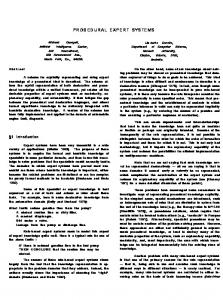
4.3.4 The Quadratic Equation Solver through Phase 3 The dependence graphs for the quadratic equation solver with the input set f a; b; c g are shown in Figure 4.12 where computations for r1 and r2 are extracted. The dependence graphs for the quadratic equation solver with a dierent 52

t=sqr(b)-4*a*c

start a==0 b!=0

r1=-c/b r2=r1

a!= 0

t>=0

11 00 00 11 00 11 00 11 DefinedRoots(a,b,c,r1,r2)

r1=(-b+sqrt(abs(t)))/(2*a) r2=-(b+sqrt(abs(t)))/(2*a)

MAIN

DefinedRoots(a,b,c,r1,r2)

Figure 4.12: Dependence Graphs for the Quadratic Equation Solver with I = fa, b, cg input set f a; b; r1 g are shown in Figure 4.13. The dependence graphs compute values for variables c and r2. The inverses of the functions sqrt and abs have been applied to derive the computations for t. The compiler can be optimized to detect that the path starting from the node computing t = ?sqr(2  a  r1 + b) can never be traversed to completion. start a==0 b!=0

a!= 0 111 000 000 111 000 111 000 111 000 111 000 111 DefinedRoots(a,b,r1, c,r2)

r2=r1 c=-b*r1

t=sqr(2*a*r1+b) t>=0

r2=(-b-sqrt(abs(t)))/(2*a) c=(sqr(b)-t)/4*a

t=-sqr(2*a*r1+b) t>=0

r2=(-b-sqrt(abs(t)))/(2*a) c=(sqr(b)-t)/4*a

DefinedRoots(a,b,r1, c,r2)

MAIN

Figure 4.13: Dependence Graphs for the Quadratic Equation Solver with I = fa, b, r1g 53

Figures 4.12 and 4.13 show that the same constraint program speci cation can be reused to derive the dependence graphs for dierent input sets. However, not all input sets can lead to dependence graphs where no constraints remain unresolved. For example, no dependence graph can be generated with the input set f a; r1 g because the simple constraint b  r1 + c == 0 and the constraint module call DefinedRoots remain unresolved in the main tree (The module call DefinedRoots remains unresolved because all the constraints in the tree for the module remain unresolved.). Note that phases 1 and 2 need not be repeated when a new input set is supplied for a constraint speci cation. Part of the appeal of a constraint programming language is its multi-directional nature - the facility to extract values for dierent sets of variables depending on the composition of the input set. While this is a secondary aspect for parallel programming concerns as compared to the ease of use aspect, this is still important in many application domains.

4.3.5 Single Assignment Variable Programs The compilation process generates dependence graphs with single assignment variables. This occurs because a child node in the dependence graph G inherits the known set of its parent as its initial known set and no deletions are made to the known set of a node. Hence, once a variable is added to the known set of a node it is retained in the known sets of all nodes in the subgraph rooted at that node. If a path in G contains nodes in the order v1  : : : vn  , where v1  is the start node, vn is the leaf and n is the length of the path, exactly one node vi  , 1  i  n, can contain a computation for a variable x. There will be no occurrence of x in any computation or ring/routing rule for nodes in v1  : : : vi?1  or in any ring rule for vi . While single assignment variables are appropriate for parallel programs, they can lead to excessive use of memory in some circumstances. Chapter 5 details our 54

approach to introduction of mutable variables where they are necessary.

4.3.6 Generation of either Eective or Complete Programs The presence of the OR operator in a constraint system results in the possibility that there exists more than one assignment of values to the variables which will result in satisfaction of the constraint system. (A given input set for a program with an OR operator may or may not allow multiple assignments which satisfy the constraint system.) A program which is eective generates exactly one set of assignments of values to variables which satis es the constraint system. A program which is complete generates all of the sets of assignments of values to variables which will satisfy the constraint system. The compilation process can be directed to generate the executable either for exactly one \OR branch" of the dependence graph or to generate the executable for all paths which lead to valid assignments. Thus, the compilation process can produce programs which are either eective or complete. A program which is complete realizes OR parallelism, as will be further discussed in Section 4.3.7. Non-determinism arises if the compiler randomly chooses a path for execution in eective programs.

4.3.7 Extraction of parallelism Our constraint representation maps to a dependence graph which is a parallel computation structure because all nodes that are enabled for execution may be executed in parallel. The constraint representation allows the targeting all types of parallelism (AND/OR, task and data parallelism) through a single representation. AND/OR parallelism refers to parallelism in computations extracted from terms connected by AND and OR operators, respectively. Task parallelism refers to parallelism in computations for dierent data. Data parallelism refers to parallelism in computations for dierent parts of a structured data item. In our system data parallelism 55

arises from the hierarchical representation of our type system. For example, matrices can be represented as blocks of sub-matrices and constraints over sub-matrices are translated to data-parallel conditionals/computations. The dierent sources of parallelism and their respective types in the representation were detailed in [JB96b] and are enumerated as follows. While 1-4 are extracted by the current compiler, 5 has not yet been implemented. 1. OR, Task: OR parallelism corresponds to executing the dierent paths in the dependence graph in parallel. These paths have resulted from the extraction of computation from constraints connected by OR operators. 2. AND, Task: The computational statements that are assigned to a node have the potential for parallel execution. For instance, the assignments r1 = (?b + r)=2  a and r2 = ?(b + r)=2  a in Figure 4.12 can be done in parallel. Parallelism is exploited by keeping in mind that the compiler generates a single-assignment system and the lone write to a variable will appear before any reads to it. A particular node may be split into several nodes to exploit the parallelism in the computations at the node. The granularity of such a scheme depends on the complexity of the functions and the operators invoked in the statements. We illustrate AND-OR parallelism in 1 and 2 through a simple example. Consider the constraint speci cation in Figure 4.14 for a program involving variables f a,b,c,x,y g. a) S2 AND/OR FOR (i < Bs2 (2) >) S2 .. . AND/OR FOR (i < Bs2 (p2 ) >) S2 .. . AND/OR FOR (i < Bsq (pq ) >) Sq There are several options available for resolution of each type of unresolved constraint. We shall enumerate some of these. 1. Since there is a 1-1 mapping between nodes in T and the dependence graph G, there is a unique leaf in G corresponding to the leaf in P containing the unresolved constraints. In Figure 4.18 the two corresponding leaves in T and G are shaded. The shaded leaf in G can be deleted. This virtually removes P from T and corresponds to not attempting to satisfy the constraint system through the path P . If deletion of the leaf in G results in its parent becoming a leaf, the parent must be deleted too. This must be continued in a recursive fashion until the deletion of a leaf does not result in its parent becoming a leaf. Then a new path descending T is chosen and pursued to see if a usable G can be obtained. This approach can be applied to unresolved constraints of any type ((i)-(iv)). Of course, there is the danger of getting an empty dependence graph if all leaves in T contain unresolved constraints. 61

T

G

P

unresolved constraints

delete

Figure 4.18: Deletion of a Path with Unresolved Constraints

2. The user may have incorrectly speci ed the initial input set by overlooking

the inclusion of some variables or including the wrong variables and may be helped in the choice of a new input set through display of the unresolved constraints and the unknowns in them. The depth- rst traversal in phase 3 can be performed again with the new input set. This can be done repeatedly until all constraints in the system are resolved. While selection of unknowns to be added to the initial input set may be easy for constraints of types (i), (ii) and (iii), it may be quite dicult to do for constraints of type (iv) since unknowns could typically be of the form A[fn1 (i1 ; : : : ; ik )] : : : [fnl(i1 ; : : : ; ik )] where i1 : : : ik are indices for nested indexed sets containing the unresolved constraints, fn1 : : : fnl are arithmetic functions over the indices, and A is any structured data type. Some parts of A may be known and other parts of A may be unknown forcing the user to identify the regions that the term A[fn1 (i1 ; : : : ; ik )] : : : [fnl (i1 ; : : : ; ik )] refers to and denote them as known. 3. Commercial solvers such as MATLAB can be invoked to solve the unresolved constraints by providing a wrapper around the invocation to the MATLAB solver in the form of a constraint module call. This technique can be most bene cial for the resolution of constraints of types (i) and (ii). 4. Iterative solutions can be attempted for unresolved constraints of types (i), (iii) and (iv) through several relaxation methods. This process is described in 62

detail in Chapter 5.

4.4 Phases 4 and 5: Speci cation of Execution Environment and Mapping to Code Apart from the textual constraint program the programmer is encouraged to specify an execution environment speci cation which is used by the compiler to optimally select certain execution environment characteristics used by CODE [NB92] to generate programs. The execution environment speci cation merits a separate discussion and is described in Chapter 6. Our target for executable for constraint programs is the CODE parallel programming environment. CODE takes a dependence graph as its input. The form of a node in a CODE dependence graph is given in Figure 4.7. It is seen that there is a natural match between the nodes of the dependence graph developed by the constraint compilation algorithm and the nodes in the CODE graph (see Appendix A for a description of CODE). The arcs in the dependence graph in CODE are used to bind names from one node to another. This is exactly the role played by arcs in the dependence graph generated by our translation algorithm. CODE produces sequential and parallel C programs for a variety of architectures. The control ow for the entire compiler is shown in Figure 4.19.

4.5 Procedural Parallel Programs for the BTS and BOER Systems In this section we show how all of the parallelism in the BTS (Figure 3.4) and BOER (Figure 3.8) examples can be extracted by the compiler.

63

Phase 1 START Constraint specification Input Set

Phase 2

Phase 3

Unresolved constraints ? Yes Delete paths with unresolved constraints?

No

Yes No Dependence graph

Change input set ? Yes

No Dependence graph

Iterative Solution Dependence graph

Mapping to CODE CODE data structures

Generate sequential/parallel programs Program

Figure 4.19: Control Flow for the Constraint Compiler

4.5.1 The BTS System Consider the speci cation for the BTS system being compiled with the input set f S0 ; : : : ; S3 ; M10 ; M20 ; : : : ; M32 ; B0 ; : : : B3 g. The speci cation has been repeated in Figure 4.20 with certain terms ( fX0 ; X1 ; X2 ; X3 g ) in bold-faced to indicate terms that are chosen as outputs by the compiler. By applying technique 3 in Section 4.3.7 the compiler splits up the speci cations to perform the multiplications in series such as M10  X0 , M20  X0 , and M30  X0 in parallel. Thus the vector multiplications for all M s within a column may be done in parallel. Figure 4.21 shows the form of the extracted data ow and exactly corresponds to the parallel algorithm in [DS86]. Data parallelism could be used on the block level operations and captured in our representation with an 64

PROGRAM BTS 1 ( S0  X0 == B0 AND M10  X0 + S1  X1 == B1 AND M20  X0 + M21  X1 + S2  X2 == B2 AND M30  X0 + M31  X1 + M32  X2 + S3  X3 == B3 )

Figure 4.20: Constraint Speci cation for the BTS System with Computed Terms in bold appropriate type structure, if desired.

4.5.2 The BOER System The constraint speci cation for the BOER system has been repeated in Figure 4.22 with certain terms in bold-faced to indicate computed terms. Each indexed set is compiled to a loop iterating over values of the index. Each simple constraint is compiled to a computation for a term (bold in Figure 4.22). Analysis of the computations extracted shows that, in the reduction phase, the computations for BP [j ]; CP [j ], and dP [i  pow(2; j )][j ] can be executed in parallel. However, dierent iterations of the loop enclosing these computations (for index j ) cannot be done in parallel due to interdependencies between the three computations. The dierent iterations of the nested loop for index i enclosing the computation for dP [i  pow(2; j )][j ] can be performed in parallel. The nested loop for index i in the back-substitution phase enclosing the computation for x[: : :] can be performed in parallel. However, the iterations for the outer loop for index j enclosing the computation for x[: : :] cannot be parallelized. Our compiler detects all the dependencies for this analysis and correctly extracts all the existing parallelism in the speci cation. 65

start Solve for X0

M10*X0

M20*X0

M30*X0

Solve for X1

M21*X1

M31*X1

Solve for X2

M32*X2 Solve for X3

stop

Figure 4.21: Dependence Graph for the BTS Program The resulting dependence graph is shown in Figure 4.23 and exactly corresponds to the data ow in the algorithm in [LD90]. The START and STOP nodes initiate and terminate the program, respectively. A FOR node initiates the dierent iterations of a loop. The two such nodes in the gure correspond to the two outer indexed sets for index j in the reduction and back-substitution phases in the constraint speci cation. The annotation \Replicated" on the arcs specify that the annotated arc and the destination node (shaded in Figure 4.23) are dynamically replicated for parallel execution. The two such annotated arcs correspond to the two nested indexed sets (for index i) in the constraint speci cation and are instances of data parallelism. The nodes annotated by BP, CP, dP, and x compute values for parts of the corresponding variable. The parallel execution of the computations for BP, CP, and dP is an instance of task parallelism. The nodes annotated by \Merge" collect computed results from parallel executions. It is to be noted that our compiler automatically detects the parallelism in the for loops in the reduction 66

and back-substitution phases. Furthermore, it is capable of extracting the parallelism within the expression 2  CP [j ? 1]  CP [j ? 1] ? BP [j ? 1]  BP [j ? 1] in the computation for BP [j ] by computing the products 2  CP [j ? 1]  CP [j ? 1] and BP [j ? 1]  BP [j ? 1] in parallel. By incorporating calls to BLAS routines (technique 5 in Section 4.3.7) which invoke parallel algorithms, incorporating data parallelism, for matrix-matrix multiply the compiler would have extracted all the existent parallelism in the example.

67

PROGRAM BOER BP[k-1] * x[pow(2,k-1)] == dP[pow(2,k-1)][k-1] AND AND FOR (j 1 k-1) f 2 * CP[j-1] * CP[j-1] == BP[j] + BP[j-1] * BP[j-1] ,

CP[j] - CP[j-1] * CP[j-1] == 0 , AND FOR (i 0 pow(2,k-j)-2) f CP[j-1] * ( dP[i*pow(2,j) + pow(2,j-1)][j-1] + dP[i*pow(2,j) - pow(2,j-1)][j-1] ) == dP[i*pow(2,j)][j] + BP[j-1] * dP[i*pow(2,j)][j-1] gg AND AND FOR (j k-1 1) f AND FOR (i 0 pow(2,k-j)-1) f CP[j-1] * ( x[(i+1)*pow(2,j)] + x[i*pow(2,j)] ) == dP[(i+1)*pow(2,j)-pow(2,j-1)][j-1] BP[j-1] * x[(i+1)*pow(2,j)-pow(2,j-1)] gg

Figure 4.22: Constraint Speci cation of the BOER System with Computed Terms in bold

68

START

FOR

CP[j]

ed

at

lic

ep

R

BP[j]

Reduction

dP[*][j]

Replicated for parallel execution

MERGE

Single-Solution

x[*]

FOR

Replicated Back-Substitution

x[*]

Replicated for parallel execution

MERGE

STOP

Figure 4.23: Dependence Graph for the BOER Program

69

Chapter 5

Iterative Solutions for Constraint Systems with Cycles Chapter 4 detailed the basic compilation algorithm for translating a constraint speci cation along with an input set to a dependence graph. The basic compilation algorithm cannot resolve constraint speci cations with input sets that give rise to dependencies with cycles. To illustrate dependencies with cycles, consider the constraint program shown in Figure 5.1. Phase 2 of the compiler collects constraints connected by AND operators at the same node and since there is only a single AND operator in the speci cation in Figure 5.1, phase 2 will generate a single node with the two simple constraints: a + b == x and x + b == y (shown in Figure 5.2). When this node is traversed in phase 3 with the input set f a; y g both simple constraints remain unresolved because there are two unknowns b and x in each of them (simple constraints are resolved as conditionals if they have no unknowns and as computations if they involve an equality and only one unknown; otherwise they are unresolved). The term cyclic is used to refer to this situation because a cycle exists in the lowlevel constraint graph representation (introduced in Section 2.3) for this constraint 70

program as shown in Figure 5.3. Note that the arcs connected to the input variables a and y have directions on them to denote that the values for these variables are available. The non-input variables x and b are in a cycle and neither of the two \+" operator nodes can \ re" for computed values to be propagated along the arcs until either x or b is given a value. The constraints involved in such a situation are sometimes referred to as cyclic constraints. In fact, cyclic constraints give rise to cyclic dependencies. PROGRAM CYCLIC DEP1 VAR int a, b, x, y; INPUTS a, y;

a + b == x AND x + b == y Figure 5.1: Constraint Speci cation and Input Set with a Cyclic Dependency

a + b == x x + b == y Figure 5.2: Tree from Phase 2 for Constraint Speci cation in Figure 5.1 This chapter discusses the augmentation [JB97] to the basic compiler for handling constraints with cyclic dependencies. We opt to use the technique of relaxation whereby iterative solutions to cyclic constraints are sought. Relaxation attempts to satisfy all the constraints in the system within a certain degree of accuracy by making an initial assignment of values to the unknowns, computing the value of one unknown in each constraint and then estimating the error in the current value. Further iterations of computing the value of the unknown variables are initiated if the errors are not suciently small. In each iteration, the values 71

a

x

+

y

+ b

Figure 5.3: A Constraint Graph with a Cycle computed in previous or current iterations are used to recompute the values of the unknowns in an attempt to achieve convergence where the dierence in computed values in two consecutive iterations is reasonably small. The solutions extracted for the unknowns in the system are often approximate. The class of numerical applications which can be solved through iterative methods is quite large. Many such applications are also quite amenable to parallelization. Relaxation is not, however, a universally satisfactory solution. Iterative methods may suer from numerical stability problems. Systems using these methods might fail to terminate. Even for systems guaranteed to converge, these methods may be very slow. A number of issues arise with respect to implementation of relaxation as an algorithm for resolution of cyclic dependencies: (i) Since there will be more than one unknown term in an unresolved constraint, how is the term to be computed selected from among all the unknown terms ? (ii) How does the compiler deal with the memory requirement for single assignment variables (Section 4.3.5) in iterative solutions ? (iii) How is the choice between the dierent kinds of relaxation methods (Jacobi, Gauss-Seidel etc.) made ? In the following sections in this chapter we trace the design of the compiler for iterative solutions to cyclic constraint systems. 72

5.1 Selection of Term to be Computed Constraints that remain unresolved through the basic constraint compiler are collected at the leaves of the tree from phase 2 and will involve more than one unknown term (except in the case of simple constraints not involving an equality). The compiler chooses one of the unknown terms in an unresolved constraint as the term to be computed and either assigns default initial values to other unknown terms or accepts such values as inputs from the user. Unresolved constraints can be of three types: a simple constraint, a constraint module call, or an indexed set of constraints (See Section 4.3.8 for a detailed description of the causes for these constraints being unresolved). The following subsections detail the selection of the computed term for the three types of unresolved constraints.

5.1.1 Unresolved Simple Constraints Relaxation can be attempted only for simple constraints involving an equality since other types of simple constraints must be resolved as ring/routing rules. An unresolved simple constraint involving an equality has more than one unknown variable and any such variable is randomly chosen as the term to be computed. For example, consider the unresolved constraints in Figure 5.2. There are two unknowns b and x in both the constraints. b can be chosen as the term to be computed in the rst constraint a + b == x. Subsequently, second constraint x + b == y has just one unknown x, which is chosen as the term to be computed.

5.1.2 Unresolved Constraint Module Calls An unresolved constraint module call has more than one unknown in its set of actual parameters, local variables and global variables in the body of the constraint module. An unknown in an actual parameter implies than the corresponding formal parameter is unknown. A constraint module call could be unresolved for either of 73

the two following reasons. (a) The tree from phase 2 for the constraint module call has unresolved constraints at the leaf of at least one path. This situation is shown in Figure 5.4(a) where the unresolved constraint C contains unknown variables f f1 : : : fp; l1 ; : : : lq ; g1 : : : gr g, where fi, 1  i  p, is a formal parameter for the constraint module, li , 1  i  q, is a local variable for the constraint module, and gi , 1  i  r, is a global variable in the body of the constraint module. Depending on the structure of C (simple constraint/constraint module call/indexed set) an unknown variable will be chosen for computation and other unknown variables will be given initial values. (b) Some subset of the set of constraints ek1 == Z1 , ek2 == Z2 , : : :, ekp == Zp (See Section 4.3.3 for a description of the terms and notation) to be resolved as computations for the child node of the call node in the dependence graph which invokes the constraint module remain unresolved (see Figure 5.4(b)). Again, depending on the structure of each unresolved constraint a computed variable is chosen and other unknown variables are initialized. T mod

G

CallNode Receives Computed Values

unresolved constraint C

Computations for ek1 == Z1 ... ekp == Zp

Tree from phase 2 for Module Call

(a)

Dependence Graph where Module is invoked (b)

Figure 5.4: An Unresolved Constraint Module Call

74

5.1.3 Unresolved Indexed Sets Relaxation cannot be used when an indexed set AND/OR FOR (i ) fA1 ; A2 ; : : : ; Ang is unresolved for the following reason (See (c) in Section 4.18).  During the resolution process a constraint Ai, 1  i  n, is resolved as a computation for some values of i in b1 : : : b2 and as a conditional ( ring/routing rule) for other values of i in b1 : : : b2. We showed in Section 4.3.8 how the compiler can generate a closed form solution in the preceding situation. If this case does not arise, the failure to resolve an indexed set of constraints can be recursively traced to \culprit" (unresolved) simple constraints and constraint module calls nested in it (Ai , 1  i  n). Consider any unresolved (simple constraint/constraint module call) constraint C nested within an unresolved indexed set. A term in C is typically of the form A[fn1 (i1 ; : : : ; ik )] : : : [fnl(i1 ; : : : ; ik )] where i1 : : : ik are indices for nested indexed sets containing C , fn1 : : : fnl are functions over the indices, and A is any structured data type. Some parts of A may be known and other parts may be unknown depending on the initial input set and the preceding computations in the current path in the dependence graph. The compiler evaluates each term in C to determine the term that accesses the largest unknown region in the structured data type. To illustrate this, consider an example constraint speci cation involving a 1  N array x in Figure 5.5. The end elements of A (shaded in Figure 5.6) are the inputs to the system. The values for the index i in the indexed set are in the range 2 : : : N ? 1. The constraint x[i ? 1] == x[i] ? x[i + 1] remains unresolved because there is no unique unknown term for all values of i in 2 : : : N ? 1 (Reason (b) in Section 4.18). The term x[i ? 1] accesses the region between indices 1 : : : N ? 2 in the array x, the term x[i] accesses the region between indices 2 : : : N ? 1 in the array x, and the term x[i + 1] accesses the region between indices 3 : : : N in the array x (see Figure 5.6). Hence, the term x[i] accesses the largest unknown region in x, i.e., 75

x[2]; x[3]; : : : ; x[N ? 1] and is selected as the term to be computed in the iteration process while other terms have to be given initial values for the rst iteration. PROGRAM CYCLIC DEP2 VAR x; INPUTS x[1], x[N]; AND FOR (i 2 N-1) f x[i-1] == x[i] - x[i+1] g Figure 5.5: Example of an Unresolved Constraint Speci cation

1

2

3

N-2 N-1 N

x[i-1] x[i] x[i+1]

Figure 5.6: Regions of Access by Terms in Figure 5.5 The motivation behind using the heuristic of selecting the term accessing the largest unknown region as the computed term is due to the following reasons.  Since the selected (computed) term accesses the largest unknown region, the largest number of values will be computed in each iteration of the relaxation process.  Since the other terms access smaller unknown regions, fewer initializations will have to be done. If the selected term does not access the entire unknown region in the data, the iterative process will not converge because certain locations in the data will not be computed. The compiler can abort the process after a xed number of iterations, 76

which can be a parameter in the system. Also, if the selected term accesses a location that is an initial input to the system, convergence may not be reached because that location will be overwritten in the rst iteration.

5.2 Mapping single assignment variables to mutable variables To satisfy a constraint within some degree of accuracy, the values for the selected unknown terms have to be computed over some number of iterations t. Since the basic compilation process generates single assignment variables, iterative computations would require t memory locations for each computed term. Such a memory requirement can be quite prohibitive when the values of large data structures are being computed iteratively. To overcome the large memory requirement for computing iterative solutions with single assignment variables, a procedure for local introduction of mutable variables is required. For each variable x being computed iteratively, the compiler may keep two locations: x and old x. Any computed value is stored in the location x. Accessed values may come from either x or old x, depending on the relaxation scheme being used. This will be detailed in Section 5.3. At the end of each iteration, a check is done to see if the dierence between values in x and old x is greater than the speci ed degree of accuracy for solution of the constraints. If it is, x is copied to old x and further iterations are initiated. The parallel functional language SISAL employs a variant of this technique [Szy91]. In our system, the user may choose to supply a value for the degree of accuracy or accept the default value assigned by the system. Using only single assignment variables, any computed variable with N memory locations would require t  N memory locations for t iterations. By transforming 77

single assignment variables to be mutable variables, the memory requirement is reduced to 2  N .

5.3 Relaxation Methods Relaxation methods such as Jacobi and Gauss-Seidel [FJL+ 88] can be used for iterative solutions to constraints. The Jacobi method is a stationary, iterative, method typically used for solving a partial dierential equation on a numerical grid. The update of each grid point depends only on the values at neighboring grid points (de ned by a stencil) from the previous iteration. In the Gauss-Seidel method the most recent grid values are used in performing updates. To generalize these two techniques to an iterative system, the Jacobi method can be implemented by using values from the previous iteration and the Gauss-Seidel method can be implemented by using the most recent values (some possibly from the current iteration). The Jacobi method yields more parallelism since all computations in a current iteration are independent. However, convergence is typically slower than the Gauss-Seidel method. The user should be able to choose the method of relaxation to be used by the constraint compiler. As mentioned in Section 5.2, two locations for each computed variable x are kept: x and old x. If the chosen method of relaxation is Jacobi, the compiler restricts all accessed values of the variable x to be retrieved from the location old x, which stores the values of variable x computed in the previous iteration. If the chosen method of relaxation is Gauss-Seidel, the compiler restricts all accessed values of variable x to be retrieved from location x which stores the most recently computed value. The compiler currently implements only the Jacobi relaxation technique.

78

5.4 The Laplace Equation Example Consider the Laplace equation for a 4-point stencil on an N  N grid indexed by (0 : : : N ? 1)(0 : : : N ? 1) as shown in Figure 3.9. A constraint speci cation for the problem was presented in Figure 3.10. The Laplace equation speci cation with the input set (boundary elements) constitutes a cyclic dependency. Applying the technique described in Section 5.1, x[i] will be chosen as the term to be computed since it accesses the largest unknown region, i.e., all interior elements in the grid x. The two indexed sets in the speci cation are compiled to loops and the simple constraint 4  x[i][j ] ? x[i ? 1][j ] ? x[i + 1][j ] == x[i][j ? 1] + x[i][j + 1] is compiled to a computation for x[i] : x[i][j ] = (x[i ? 1][j ] + x[i + 1][j ] + x[i][j ? 1] + x[i][j + 1])=4. If the Jacobi method of relaxation is chosen by the user, the constraint speci cation can be compiled to the procedural code shown in Figure 5.7. If the GaussSeidel method of relaxation is chosen by the user, the constraint speci cation can be compiled to the procedural code shown in Figure 5.8. The user may supply initial values for the interior (non-shaded) points of the grid or choose to accept the default initial values assigned by the compiler. Variable x is initialized to the initial values and the input boundary values. Variable old x is initialized such that at least one point diers in value from its corresponding point in x by more than the degree of accuracy so that the rst iteration can be initiated. The function check accuracy(x, old x) returns 1 if the dierence between any value in x and old x is greater than the degree of accuracy; otherwise it returns 0. The function copy values(old x,x) copies values from locations in x to corresponding locations in old x.

5.4.1 The Dependence Graph for the Laplace Equation Compilation of cyclic dependencies for an iterative solution has been implemented in the constraint compiler for the Jacobi method of relaxation. The Gauss-Seidel 79

while (check accuracy(x,old x)) f copy values(old x,x); for (i 2 N-2) f for (j 2 N-2) f x[i][j] = (old x[i-1][j] + old x[i+1][j] + old x[i][j-1] + old x[i][j+1])/4

ggg

Figure 5.7: Jacobi Relaxation for the Laplace Equation while (check accuracy(x,old x)) f copy values(old x,x); for (i 2 N-2) f for (j 2 N-2) f x[i][j] = (x[i-1][j] + x[i+1][j] + x[i][j-1] + x[i][j+1])/4

ggg

Figure 5.8: Gauss-Seidel Relaxation for the Laplace Equation method has not yet been implemented. In the Jacobi method of relaxation, both loops (for i and j ) surrounding the computation can be executed in parallel. A naive parallelization of the loops will lead to (N ? 2)2 computation nodes, each executing an instance of the computation x[i][j ] = (old x[i ? 1][j ] + old x[i + 1][j ] + old x[i][j ? 1] + old x[i][j + 1])=4. This is highly undesirable since the computations are too ne-grained. To overcome this, the compiler detects instances of computation extracted from constraints speci ed at the scalar level. Simple data partitioning techniques are applied to partition the data involved in the computation over a speci ed number of computation nodes P . The data partitioning techniques will be detailed in a later chapter. In the Laplace equation, the grid x is partitioned in a row-wise manner across P nodes in the extracted dependence graph. Each partitioned slice in a computation node contains locations that the node computes through each iteration and any overlapping regions 80

with other computation nodes that it accesses. For computations speci ed at the scalar level, as in this case, the region of overlap between computation nodes is determined by examining the terms in the computation. In the Laplace equation, the accessed terms are x[i ? 1][j ]; x[i + 1][j ]; x[i][j ? 1]; and x[i][j + 1]. The indices for the accessed terms specify a maximum displacement of 1 in the four directions of north, south, east, and west. Since x has been partitioned in a row-wise manner, the overlap is 1 row in the north and south directions. The row-wise partitioning of a 10  10 matrix across 4 nodes numbered 0 : : : 3 is illustrated in Figure 5.9. Each node i, 0  i  3, gets rows in the range 2  i : : : 2  (i + 1) + 1. 0 1 2 3

0 1 2 3 4 5 6 7 8 9 0 1 2 3 4 5 6 7 8 9

Figure 5.9: Data Partitioning for the Laplace Equation In Figure 5.10 we show the dependence graph extracted by the compiler for a Laplace equation system executing on P nodes. The super node S initiates new iterations. The computation nodes numbered 0 : : : P ? 1 each have a slice of approximate size NP P + 2 (overlap between slices) of the matrix x. In each iteration the code in Figure 5.7 is executed by each computation node on its local slice. At the end of each iteration overlapping regions are exchanged between computation nodes and the super node is informed by each computation node whether the degree of accuracy has been reached for the values in the local slice. Computation is terminated when all the nodes achieve convergence on individual slices. 81

S

0

1

P-1

Figure 5.10: Dependence Graph for the Laplace Equation

82

Chapter 6

Execution Environment Speci cation The advantage of using a program speci cation that is independent of the execution machine is portability - the ability to create executables for dierent architectures without changing the program speci cation. The constraint program speci cations in our system are translated to an intermediate architecture-independent dependence graph which can be mapped to many dierent parallel machines. However, there are many architectural mechanisms which can be exploited by an executable program if it is directed to do so. This usually leads to an improvement in performance. Without violating the \sanctity" of our architecture-independent program speci cation, we propose an execution environment speci cation, separate from the constraint program, that allows the user to provide useful hints to the compiler about the underlying execution machine. The compiler can use these hints to produce programs that may be more optimized for performance. This chapter discusses the design of the execution environment speci cation for our compiler. Several features are discussed in individual sections. While some of them have been implemented in our system, there are several others which could 83

be added in the future.

6.1 Shared Variables In shared memory architectures such as the Sparc and Cray J90, a vast improvement in performance can be obtained if some variables are declared as shared because it avoids the copying of large data across computation nodes. This is demonstrated through the BTS example in a later chapter where performance results for a version of the program not using shared variables and another using shared variables are presented. The program using shared variables shows a dramatic improvement in performance over the one not using shared variables. The user has to be cautious when declaring shared variables in a program containing constraints connected by OR operators. OR operators translate to multiple paths in the dependence graph and hence, give rise to the potential for multiple solutions. In a program not using shared variables, each path can compute a solution independent of other paths. However, a path in the dependence graph for a program using shared variables may overwrite the value computed for a variable in another path. To illustrate this, consider the dependence graph in Figure 6.1 where both paths emanating from the start node will be executed if c > 0. If a and b are shared variables instead of being local to each node, only one solution for a and b will be nally retained and it could be one of fa = 10; b = 20g, fa = 10; b = 0g, fa = 5; b = 20g, and fa = 5; b = 0g depending on the interleaving of computations in a parallel environment. However, since nodes in CODE lock shared variables when execution is started and the locks are released only after the entire computation is completed, only one of the two solutions - fa = 10; b = 20g and fa = 5; b = 0g- is possible in our system. Hence, the user should not declare variables as shared if there is the potential for multiple solutions for them, which can be determined from the constraint 84

start c>=0

c!=0 a=10 b=20

a=5 b=0

stop Figure 6.1: A Dependence Graph with Multiple Solutions speci cation by inspection.

6.2 Number of Available Processors This piece of information can be used to determine the number of nodes to be created when spawning o a computation to be executed in parallel. For example, the N iterations in a loop structure can be partitioned across P processors such that each processor gets approximately NP iterations to execute or the data computed within a loop structure can be partitioned equally across P processors. Since CODE allows the dynamic creation of nodes, the number of processors can determine the number of computation nodes at runtime.

6.3 Data Partitioning with Overlap Sections It has been amply demonstrated by many parallel programming experiments that data partitioning techniques play a signi cant role in improving performance. While, currently, we have only implemented simple mechanisms for data partitioning, we show in this section that other sophisticated mechanisms can be speci ed too. In many applications such as the Laplace equation, the computations are 85

speci ed at a very ne granularity, say, at the scalar level. When the compiler detects that the operations involved in the computations are over scalar types or over smallsized data (the threshold size is xed by a parameter to the system), it partitions the variables involved over a number of nodes. This is especially important if the computation is nested within loops because the computation is executed repeatedly and the overhead in executing scalar operations repeatedly can severely degrade performance. The form of the partition depends on the data accesses in the computation. For any matrix, if the accesses are only in the north and south directions the data is partitioned column-wise. If the accesses are only in the east and west directions the data is partitioned row-wise. If there are accesses in mixed directions, say north and east, the data is partitioned such that there is minimum overlap between the partitioned slices. This scheme minimizes the overhead in the synchronizations necessary when data is shared across computation nodes. Each node gets approximately N M + overlap, where the matrix being partitioned is of size N  M and P is the P number of nodes. The amount of overlap between partitioned slices must be determined by the user or by the compiler by inspecting the terms in the computation. The mechanism of partitioning data involved in scalar computations has been used for the Laplace equation. The user may specify the partitioning mechanism, instead of allowing the compiler to select it, by indicating the actual regions in the data type to be distributed across the nodes. (The user must specify the actual overlap between the partitions to determine the regions to be synchronized.)

6.4 Option of not Parallelizing a Module A constraint module may have very ne-grained operations in the constraints for the constraint module body. Parallelizing such a module may lead to degradation in 86

performance due to the overheads involved. For this reason, a user can denote that the dependence graph for a particular module call should be mapped to a sequential procedure rather than a parallel one. This feature has not yet been implemented in our compiler. However, since CODE allows the generation of sequential programs, this would be simple to incorporate.

6.5 Selecting Operations to be Executed in Parallel Operations over structured data types are primitives in the type system. But parallel execution can be selected for these primitive operations. The complexity of some of these operations may be larger than others. An example is the matrix-matrix multiplication operation. In the interests of performance, it would be bene cial to extract such operations out of a computation to execute in parallel. For example, if there is a computation (d1 4 d2 ) 5 (d3 4 d2 ), where 4 and 5 are primitive operations, to be executed and the operation 4 is very computation-intensive, the speci cation can be split into two computations to be executed in parallel: (d1 4 d2 ) and (d3 4 d2 ). The results can then be merged and operator 5 can be applied on them. We use this technique in the BTS example where multiple matrix-matrix multiply operators in a computation are executed in parallel. The execution environment speci cation provides a platform for the user to indicate that some operations be selected for extraction from a computation for subsequent parallel execution.

6.6 Choices among Parallel Algorithms to execute some of the Operations A variety of choices exist among parallel algorithms to execute operations on data instances under a type system. The user should be able to select one among a 87

number of implemented algorithms in the system to execute an operation. We have not yet implemented this feature in our system.

88

Chapter 7

Performance Results A prototype of the constraint compiler has been implemented in C++ using objectoriented techniques. A number of examples have also been programmed and executed on the Cray J90, SPARCcenter 2000, Enterprise 5000, Sequent Symmetry machine [Ost89], and the PVM system. The sections in this chapter present the performance results obtained for some of the examples programmed in our system. Overall, the results have been extremely satisfactory. The execution times reported in this chapter are wall clock times. Whenever possible, timings have been taken for executions during either dedicated CPU access or when the loads on the machines were low.

7.0.1 The Block Triangular Solver (BTS) The extracted dependence graph corresponds to the parallel algorithm in [DS86]. The parallelism yields an asymptotic (in the number of blocks) speedup of N 2 =(3N ? 2), where N is the number of blocks. Asymptotic speedup assumes zero communication and synchronization times. Figure 7.1 gives the speedups for a 1200  1200 matrix on a 14-processor shared memory Sequent machine. A hand-coded parallel program was written by 89

another student in connection with experiments on the CODE system. It is seen that the performance of the constraint generated code is comparable to the handcoded program's performance. The dierence in speedups is mainly due to the fact that the hand-coded program is optimized for a shared memory execution environment. These results were obtained with an earlier version of the constraint compiler before any provision for speci cation of execution environments was implemented. The Sequent computer system was no longer available by the time the optimizing compiler had been developed. BTS Performance on Sequent 4.5 Constraint Asymptotic Hand

4 3.5

Speedups

3 2.5 2 1.5 1 0.5 0 0

2

4 6 Number of Processors

8

10

Figure 7.1: Performance Results for BTS Program on a Sequent Figure 7.2 gives the speedups for an 8800  8800 matrix (number of blocks=11, 90

block size=800) on an 8-processor SPARCcenter2000. This program has been optimized for shared variables. It is to be noted that the constraint generated code performs quite well for the small number of processors available. The speedup is slightly higher than the asymptotic speedup until about 7 processors, after which it drops. At 8 processors the dierence in speedups between the asymptotic and the program generated from constraints is about 10%. BTS Performance on Sparc 4.5 Constraint Ideal 4

3.5

Speedups

3

2.5

2

1.5

1

0.5

0 0

1

2

3 4 5 Number of Processors

6

7

8

Figure 7.2: Performance Results for BTS Program on a SPARCcenter 2000

91

7.0.2 The Block Odd-Even Reduction Algorithm(BOER) The generated dependence graph for the BOER system (Figure 4.23) maps to a procedural program which executes the reduction, single-solution, and back-substitution phases in order. The dependence graph has been repeated in Figure 7.3 with annotations on the nodes denoting the complexity of the operations in the computations performed at the nodes. In the reduction phase, the computations for BP [j ] and CP [j ] are of complexity O(n3) since they both involve matrix-matrix multiplication. All other computations in the reduction phase (computation for dP ) and the other phases (computations for x) are of complexity O(n2 ) since they involve matrix-vector multiplications.

O(n3 )

Reduction

Single-Solution

Back-Substitution

BP[j]

x[*]

O(n3 )

O(n2 )

CP[j]

dP[*][j]

Replicated for parallel execution

O(n2 )

O(n2 )

x[*]

Replicated for parallel execution

Figure 7.3: Dependence Graph for BOER Program annotated with complexity The authors in [LD90] have mentioned that the single-solution step is the 92

major bottleneck in the algorithm. But, in our experiments we found the reduction phase resistant to scalability. This is due to the fact that the computations for BP [j ] and CP [j ] are O(n3 ) operations. This dominates the scalable part of the loop: the computation of dP , which is O(n2 ). If we incorporate parallel algorithms for matrix-matrix multiplication (technique 5 in Section4.3.7), this bottleneck will be overcome. In addition, the single-solution step will also be parallelized leading to even better performance. Figure 7.4 presents the speedups over a sequential implementation of the algorithm on an 8-processor SPARCcenter 2000 for n=200 and k = 7(M = 127) and k = 8(M = 255) for the back-substitution phase of the algorithm. Note the attainment of near-linear speedup for this (relatively small) number of processors.

7.0.3 The Laplace Equation Figure 7.5 presents speedups for the solution of the Laplace Equation for an 840840 grid over a sequential implementation of the solver on a CRAY J90. Figure 7.6 presents speedups for the solution of the Laplace Equation for dierent sizes of the grid over a sequential implementation of the solver on a Sparc (Enterprise 5000) with 8 processors. Both executions used the Jacobi method of relaxation. As expected, the number of iterations for convergence was very high. Consequently, the time taken for experiments ran into several hours. The results presented here were obtained for a fairly small degree of accuracy so that the number of iterations were small. This is a reasonable setup for the experiments since each iteration took approximately the same amount of time. It can be seen that the speedups obtained for the CRAY are fairly good considering the small size (approximately 800  800) of the grid which is partitioned across the nodes. The results on the Sparc show that as the size of the problem 93

BOER Performance on SPARCcenter 2000 5.5 k=7,n=200 k=8,n=200

5 4.5

Speedups

4 3.5 3 2.5 2 1.5 1 1

2

3 4 5 6 Number of Processors

7

8

Figure 7.4: Performance Results for BOER Program on a SparcCenter 2000 increases, corresponding to an increase in the amount of computation at each node, the speedups improve. Page faults marred the results for grid sizes greater than 7500 and hence are not reported.

94

Laplace Performance on Cray J90 8 840 * 840 Matrix 7

6

Speedups

5

4

3

2

1

0 0

1

2

3

4

5

6

7

8

Number of Processors

Figure 7.5: Performance Results for Laplace Equation Program on a CRAYJ90

95

Performance Results for Laplace on Sparc 8 840*840 4200*4200 7500*7500 7

6

Speedups

5

4

3

2

1

0 0

1

2

3 4 5 6 Number of Processors

7

8

Figure 7.6: Performance Results for Laplace Equation Program on an Enterprise 5000

96

Chapter 8

Related Work Our research is related to work in two elds: parallel programming and constraint programming. The goals in these areas have been quite dierent. Constraint programming research has focussed on providing constraints as an attractive platform for sequential and concurrent programming both for general and special purpose environments. Not much emphasis has been placed on performance in concurrent constraint systems. In contrast, the parallel programming community has mainly concerned itself with performance, although many programming models have been proposed over the years. We have attempted to bridge the motivations in the two areas through this research. Parallel programming has a vast spectrum of research to its credit over the years. In comparison, constraint programming research has been modest in scope. One of the earliest constraint systems was Sketchpad [Sut63] developed by Ivan Sutherland in 1963. But, most of the work in the eld did not begin until the 1980s. However, since then there has been a urry of activity which has continued until the present day. Out of the many outstanding research projects in the two elds, we have selected those most closely related to this research for discussion.

97

8.1 Constraint Programming 8.1.1 Consul The goal of Consul [Bal90] resembles ours in that it is to extract parallelism from constraints. But the approach is dierent in that interpretative local propagation is used to nd values satisfying the system of constraints. This approach has little hope of extracting ecient programs and oers performance only in the range of programs written in logic languages. A noteworthy feature of the language is that it oers sets (with set operations) as a primitive data type.

8.1.2 Thinglab Thinglab [FB89] transforms constraints to a compilable language rather than to an interpretive execution environment. It is a constraint-oriented graphic simulation laboratory where constraints are compiled to sequential procedural code. The compilation of simple constraints is done by storing all possible transformations for a single constraint. No compilation for structures involving indexed sets or constraint modules is done. Also, the system is not concerned with the extraction of parallel structures, which is our major concern.

8.1.3 Kaleidoscope Kaleidoscope [FBB92] integrates two dierent paradigms - constraint programming and imperative programming - within the same programming language. It could be basically seen \either as adding constraints to imperative programs, or as adding control ow to constraint programs" [FB91]. Programs in the language mix objectoriented constructs with constraints. As in Thinglab, compilation to procedural code has been attempted. However, Kaleidoscope does not target parallelism and the compiled constraint structures are simple (as de ned in Section 3.3). 98

8.1.4 Concurrent Constraint Programming Vijay Saraswat described a family of concurrent constraint logic programming languages, the cc languages [Sar89]. The logic and constraint portions are explicitly separated with the constraint part acting as an active data store for the logic part. The logic communicates with the constraint part only through constraints either by a \tell" operation (a new constraint is added to the store) or an \ask" operation (to check if a constraint is consistent with the store). A number of systems based on the cc model were developed. The most notable among them is Oz which is a concurrent programming language based on an extension of the basic concurrent constraint model provided in [Sar89]. The performance reported for the system is comparable with commercial Prolog [MSS95].

8.2 Parallel Programming 8.2.1 Automatic Parallelization of Sequential Programs Attempt to parallelize Fortran with additional speci cations have not been broadly successful [EB91, PW86]. There have also been attempts to parallelize languages such as Scheme and other dialects of Lisp [LH89, HP88]. There are several algorithms for generation of ecient (optimal or near optimal) parallel code from straight-line code [MRK88]. There are a number of algorithms for fast parallel evaluation of expressions [KR90]. These algorithms can, in some cases, be applied to the sequential code segments in the macro-parallel computation structures generated by our compilation process as further optimizations or to obtain micro-level parallelism when it can be exploited by the underlying execution environment.

99

8.2.2 Extension of Procedural Languages with Directives for Parallelism There are many extensions of sequential languages with directives for parallelism. We consider only two of them in this section. Declarative extensions have been added as part of High-Performance Fortran(HPF) [Ric]. This is a data-parallel programming language designed for portability and an implicitly parallel programming style with some optimization directives. In these respects, it is similar to our system. But, the dierence lies in the program speci cation styles: procedural versus declarative. Also, HPF does not address task parallelism. CC++ [CK92] is a parallel programming language designed by providing extensions to the object-oriented language C++. It incorporates the fundamental ideas from compositional programming: synchronization variables and parallel composition.

8.2.3 Parallel Logic Programming PCN [CT92] and Strand [FT90] are two parallel programming representations with a strong component of logic speci cation. Both require the programmer to provide explicit operators for speci cation of parallelism and the dependence graph structures which could be generated were restricted to trees.

8.2.4 Parallel Functional Programming Functional languages are unidirectional (a single variable is computed) as opposed to constraint languages which are multi-directional (any variable in a constraint can be computed). A number of parallel systems have emerged from the functional programming area. Most prominent among them are SISAL, EPL, Id, Crystal, and the PTRAN system. A description of these systems can be found in [Szy91]. While 100

SISAL and Id are pure implicitly parallel languages, EPL provides mechanisms for expressing mapping and scheduling constraints. PTRAN provides explicitly parallel control structures.

8.2.5 Equational Systems Equational speci cations of computations [O'D85] are a restriction of constraint speci cations. Unity [CM89] is an equational programming representation around which Chandy and Misra have built a powerful paradigm for the design of parallel programs. Unity requires addition of explicit speci cations for parallelism.

8.2.6 Miscellaneous Systems Other related work includes technical computing environments like MATLAB [Mat83] which integrate numerical analysis and matrix computation. We, of course, use the methods of parallel compilation [Ban94] to derive procedural programs from constraint systems. The approach of Pandey and Browne [PB93] expresses parallel computation as constraints on the order of execution of units of computations. We derive this ordering from the constraints and an input set of variables. Collins [CB95] expresses matrix computations as hierarchical type declarations and translates to implementations which maximizes use of type information. We use hierarchical matrices as a tool for controlling granularity. Chapters 1 and 2 emphasized why our approach may hold greater promise for parallel programming than parallel procedural languages. Some reasons why our approach has greater potential for obtaining ecient parallel programs than parallel logic languages, compilation of functional languages to parallel execution and/or concurrent constraint logic programming languages include (i) A constraint speci cation system can provide a richer set of primitives than is given in current logic languages. (ii) Functional languages restrict data ow to be unidirectional whereas 101

constraint systems impose no constraints on data ow. (iii) Data parallelism is more readily expressed in constraint speci cations than in pure functional languages. (iv) Concurrent constraint satisfaction systems currently rely on interpretive methods for evaluation of constraint satisfaction whereas we compile to direct procedural code. (v) Narrowing the target domain and direct use of semantic domain knowledge enable the compiler to choose ecient algorithms for the derived computations.

102

Chapter 9

Conclusions In conclusion, we believe we have demonstrated that constraint programs oer a rich, relatively untapped representation of computation from which parallelism can be readily extracted. Constraint systems with appropriate input sets can be translated to generalized dependence graphs which can be mapped to parallel programs for a variety of architectures. Coarse-grain parallelism can be extracted through modularity, operations over structured types, and speci cation of atomic functions. All types of parallelism (AND, OR, task, data) can be derived. Either eective or complete programs can be derived from constraint systems on demand. Programs for dierent computations can be derived from the same constraint speci cation by dierent choices of the input set of variables. By giving the programmer control over compilation choices for the execution environment, we can assist in the generation of architecturally optimized parallel programs. This research has established that constraint systems can be compiled to ecient coarse-grained parallel programs. In fact, we have been quite surprised at the ease of attaining these results from such a radical representation.

103

9.1 Contributions The main contributions of the work are enumerated as follows. (1) We have de ned a constraint language which can satisfactorily represent a wide class of scalar and matrix-based programs. (2) We have designed and implemented a basic compilation algorithm for one class of acyclic constraints. The compiler translates a constraint speci cation and an input set of variables to a generalized dependence graph which is a parallel computation structure that computes values for the (single-assignment) non-input variables. Simple constraints are compiled to assignments and conditions, constraints connected by AND operators lead to sequencing, constraints connected by OR operators lead to branching and multiple solutions, indexed sets are compiled to loops, and constraint module calls are compiled to procedures. (3) We have developed an extended compiler to handle cyclic constraints through relaxation. This allows the targeting of many parallel iterative numerical applications such as the Laplace Equation and Partial Dierential Equation solvers. The large memory requirement for single-assignment variables in iterative systems has also been overcome. (4) We have demonstrated the feasibility of the approach to compilation of parallel programs by speci cation and execution of a number of interesting applications and demonstration of good performance results on a variety of parallel machines. (5) We have opened the path for targeting many new applications.

104

Chapter 10

Future Work Our research has established the feasibility of expressing computations for parallel execution as constraints. It also paves the way for a number of future research endeavors. In the subsections of this nal chapter, we present a few of the possible future directions for research.

10.1 Extraction of Algorithms Constraint speci cations do not explicitly specify algorithms. However, algorithms can be extracted from them by supplying appropriate input sets of variables. Our system opens up the possibility of extracting algorithms for applications where algorithms are dicult to specify. One such application is a Partial Dierential Equation Solver using domain decomposition methods where it is far easier to specify the constraints that must be maintained within a particular domain and across the boundaries of domains than to specify how to maintain these constraints. A number of issues such as the factors determining the optimality of the extracted algorithms require research.

105

10.2 Writing \Good" Speci cations An issue that has been raised is \how to write 'good' constraint speci cations". One could write a speci cation in which a large number of function calls and very few constraints are used. Take, for example, the Barnes Hut problem in parallel programming. One could express the building of the quad-tree as a call to a procedural function or a constraint module. Of course, the decision to choose one representation over the other might be based on whether or not to parallelize the particular computation. On the other hand, we can provide the capability (through the execution environment speci cation) of not parallelizing a particular constraint module. So, this decision might be based on other factors such as expressibility.

10.3 Choosing a Path in Eective Programs In Section 4.3.6 we explained how eective programs (programs with a single solution) can be extracted by the compiler through choosing only a single path in the dependence graph for execution. The choice of a path among a number of paths is based on factors such as maximal output (computed) set of variables. This needs further investigation.

10.4 Exploring New Application Areas Other application areas such as boundary matching for decomposed domains, data mediation, back tracing in circuits, and development of distributed network applications each oer opportunities for constraint speci cation systems.

106

10.5 Extensions to Current Work The current representation and compilation system are a solid feasibility demonstration. But much more could be done in the domain of matrix computations. Complete implementation of the execution environment speci cation and the full feature set for the hierarchical type system need to be done. Additionally, further steps in this research are to de ne the semantics of recursion in constraint module calls, to relax the requirement that all of the bounds in indexed sets of constraints be statically found, and to incorporate higher-order solvers for unknowns in computations.

107

Appendix A

CODE A brief discussion on the CODE graphical programming environment is presented here. A more detailed exposition of the system can be found in [NB92]. In CODE a program is graphically represented by nodes (dierent kinds) connected through arcs. CODE programs consist of a set of graphs. Graphs are its equivalent of subroutines in conventional programming languages. The formal parameters for a graph are de ned by its interface nodes (input and output) and its creation parameter nodes. A Call node in the calling graph is always bound to exactly one instance of the invoked graph.

A.1 Nodes Unit of Computation (UC) Nodes : UC nodes are CODE's basic computational unit. They extract information from incoming arcs, perform a sequential computation on it and pass out the resulting information on outgoing arcs. This process is called \ ring" and takes place under conditions speci ed by user-supplied ring rules. Each UC has its own names for the arcs incident upon it. These names are called \ports" for data ow arcs and \shared variables" for arcs that connect the UC to a 108

name-sharing relation. Nodes may have local variables and these variables retain their state from one ring to the next. Name Sharing Relation Nodes: Name sharing relations allow the controlled use of shared variables in CODE programs. Access to them is speci ed declaratively. Shared variables are de ned at Name Sharing Relation nodes. UC nodes that share the variable must have an arc drawn from them to the corresponding Name Sharing Relation node. These arcs have a topology rule that binds the shared variable name used in the Name Sharing Relation node to a shared variable name used in the UC node along with the mode of access -reader or writer (of the shared variable). Call Nodes: Call nodes are used to call one graph from another. Exactly one graph instance is bound to each instance of a Call node. Arcs that are incident on a Call node are actual parameters to the graph being called. Their topology speci cations may bind them to either an Interface node or a Creation Parameter node in the called graph. Creation Parameter Nodes: Creation Parameter nodes de ne a formal parameter to a graph that will have exactly one value bound to it in the lifetime of a graph instance. The value will be bound before the graph instance is created and becomes available as a constant throughout the graph. Interface Nodes: They de ne a graph's interface and are a type of formal parameter. They provide a name that can be referred to in an arc topology speci cation in a calling graph. Interface nodes provide aliases for ports on UC nodes when a UC node must be linked to a UC node in a dierent graph.

A.2 Arcs Arcs in CODE bind nodes together. There are two classes of arcs. Arcs that are not incident upon one or more interface nodes use arc topology speci cations to specify 109

where data are to go to given where they come from. For example, suppose a graph has a UC node called N1 with output ports Y1 and Y2 and another UC node called N2 with input ports X1 and X2. An arc drawn from N1 to N2 is ambiguous since no ports have been speci ed. An arc topology speci cation solves the problem. For example, .Y1 ) .X2 says that the arc goes from N1's output port Y1 to N2's input port X2. The rule can be interpreted in the following manner : if data come from node N1's port Y1, then they must be sent to node N2's port Y2. The node names need not be mentioned in the rule since the CODE system knows what nodes are involved from the graphical context { the user has already drawn the arc from one node to another. Arc topology speci cation may also involve indices. For example, suppose node N1 places data on its output port Y1[i] where i takes values from 0 to 9. The rule .Y1[i] ) [i].X2 says that data from N1's port Y1[i] must be sent to node N2[i]'s port X2 for all i in the range 0 : : : 9. Arcs that are incident on interface nodes do not have topology speci cations. Instead, the user must supply the name of the entity the interface node is connected to. One can think of the interface node as aliasing an entity. For example, an input interface node connected to an UC node is bound to an input port in the UC. The interface node serves as an alias for a particular port in a particular UC.

A.3 Firing rules and Routing rules Firing rules serve two purposes. They specify conditions under which the node is allowed to re, and they extract values from arcs and place them into local (node) variables. In addition, they can set local variables. A ring rule consists of guards 110

and bindings as shown. Guard1, Guard2, . . . , GuardK ) Bind1; Bind2; . . . , BindL The rule evaluates to TRUE and the node can re when all of its guards evaluate to TRUE. The commas can be interpreted as \and". For example, the following ring rules speci es that the corresponding node can re when there is data on V1 and V2 (the data is stored in n1 and n2). ring rules f V1 ! n1, V2 ! n2 )

g

Routing rules place data onto outgoing arcs and can set local variables too. Routing rules consist of guards and bindings as shown. Guard1, Guard2, . . . , GuardK ) Bind1; Bind2; . . . , BindL The rule evaluates to TRUE and its bindings will be done when all of its guards evaluate to TRUE. For example, the following routing rule speci es that the value of n+1 should be placed onto V. routing rules f TRUE ) V n+1 ;

g

A.4 Formal speci cation of CODE model The elements of the uni ed model of parallel computation are de ned in set notation in terms of the graph model, the Uni ed Computation Graph model. (Refer to [WBS+ 91] for details). Formally, a Uni ed Computation Graph (UCG), G is a tuple (S, D, E, T) where S is a set of nodes s of G D is a set of data dependencies d of G E is a set of exclusion dependencies e of G 111

T is some type system Given a countably in nite set of values U , a type system is a family of subsets of U called types. There are n distinguished subsets B1 ; : : : ; Bn of U called basic types. There is also a set of strings called identi ers or names. These subsets and strings together constitute a type system T . We write n : t if identi er n has type t. A type t is either 1. A basic type 2. U 3. (Records) The union of the sets fnamej g  tj where namej is an identi er and tj is a type, given a xed set of name and types, name1 ; ; : : : ; namen and t1 ; : : : ; tn . 4. (Arrays) If I1 ; : : : ; Im are nite totally ordered sets and t is a type then the set of functions f : I1  I2  : : :  Im ! t is a type. A port p of type t is semantically similar to an identi er with a type t (it is a node's name for a data arc incident on it). A node s has a set of input ports denoted IP(s) and a set of output ports denoted OP(s).

De nition A.1 A Data dependency d has an associated pair of nodes, s1 = Source(d), s2 = Sink(d), a type t = T(d), and a name N(d). It connects ports in s1 (called Out Port(d) 2 OP(s1)) to ports in s2 (called In Port(d) 2 IP(s1)) where either In Port(d) or Out Port(d) can be an indexed array of ports. An arc topology speci cation is used to map the data from Out port(d) to In Port(d).

Intuitively, a data dependency is a buer which carries a sequence of typed values from source to sink. We use an operator style notation; for example, if G is a UCG then S(G) is the set of nodes, D(G) is the set of data dependences of G. For a data dependency d, S(d) = f Source(d), Sink(d)g , the node set for the dependency 112

For a node s, In(s) = fd | Sink(d) = sg, Out(s) = fd | Source(d) = sg S D(s) = In(s) Out(s)

De nition A.2 A node n is a two-tuple, n( ring rule, relation). De nition A.3 A ring rule fr is a predicate over the state of the input dependencies In(s) of a node s.

De nition A.4 A routing rule rr is a predicate over the state of the local node variables that speci es how data is routed along the output dependencies Out(s) of a node s.

Intuitively, the relation is executed in nite time after the predicate of the ring rule evaluates to true. The input ports accept data from the input data dependencies as speci ed in the ring rules while its output ports route data along output data dependencies according to the routing rules.

A.5 A CODE Implementation Overview The CODE visual parallel programming system runs under UNIX and produces target code suitable for a variety of platforms and architectures, including shared and distributed memory multiprocessors. These include all UNIX-based single and multi-processor shared memory platforms with POSIX threads and networks of such systems (or multicomputers) using PVM or MPI. Targeted platforms include the Sun Sparc 20 (a uniprocessor workstation), the Sun Enterprise 5000 (an SMP with 8 processors), the Cray J-90 (an SMP with 16 processors), a network of Sun workstations communicating via PVM or MPI, and the IBM SP2 (a distributed memory multicomputer with 12 processors). 113

The distributed memory implementation of CODE is an extension of the shared memory implementation and incorporates the same basic underlying execution model, so we will initially focus on the shared memory implementation and then discuss the distributed memory extensions. CODE compiles programs by transforming computation nodes, graphs, namesharing relations and arcs into C++ procedures. These procedures implement the actual computations and data transfer. When data is transferred to a node, a hash table maintained in the graph's data structure is checked to see if that node exists; if it does not, a new one is instantiated and added to the table. The data is then transferred to the node's input port (a FIFO queue) and that node is added to the ready deque of pointers to the data structures representing computation nodes. When a CODE program is run, a user-speci ed number of worker threads 1 are spawned. The start node is added to the deque. Each of these workers repeatedly attempts to remove computation nodes from the deque (the deque is protected by a condition variable and workers are awakened only if work is available for them to execute). After popping a node, the worker tests the node's ring (input) rules. If any of these succeed, the worker executes the node's computation, tests the node's routing (output) rules and executes any succeeding rule. The worker is then available to continue executing more computation nodes. This continues until the stop node is executed, at which point all execution terminates. In CODE, shared variables are kept inside a name-sharing relation node. This node holds any number of many-readers, one-writer shared variables. Nodes which access any of these shared variables must be connected to the name-sharing relation by an arc and must declare whether they want read-only or read-write access to the shared variables. Every name-sharing relation has an associated reader queue and writer queue Kernel-level threads (LWPs in Solaris terminology) are required to ensure that threads are distributed across all processors. 1

114

along with a count of active readers and writers (that is, executing nodes with readonly access and nodes with read-write access). When a worker pops a node that uses a shared variable, it rst checks to see if it can be granted access. There are three cases: there are active readers, there is one active writer, or neither. Access is immediately granted if there are active readers and the node is a reader and there are no writers waiting, or if there are no active readers or writers. Nodes are added to the appropriate queues otherwise. When all readers or the one writer has nished execution, all of the waiting nodes are added to the ready queue to allow them to contend for the name-sharing relation. The distributed version of CODE incorporates some extensions to the system described above to allow for multiprocessor execution. All CODE computation nodes, graphs and name-sharing relations are mapped to processing elements (i.e., individual computers, regardless of the number of processors) by a straightforward algorithm. CODE objects are assigned prime numbers as unique identi ers (UIDs) and at runtime new instances of these may be created with a list of indices. A CODE object is uniquely determined by the series of UIDs and indices of all of its containing graphs, starting at the root, along with the object's own UID and indices. The distributed version of CODE computes the home processing element for each object by summing the UID's and indices of the containing graphs modulo the number of processing elements. Nodes that do not depend on any local state are called non-static nodes and are always mapped to the local processing element. All data sent to a node is routed to the home processing element. This mapping ensures that all nodes at the same level of the graph are grouped on the same processor so that creation parameters are local and communication only occurs between graphs. As long as there is sucient replication of graphs, parallelism is maximized and communication is minimized, but this cannot be guaranteed in general. 115

To remedy this, load balancing is provided using a work-stealing [BL94]. algorithm. The work-stealing algorithm used guarantees asymptotically ecient execution of certain CODE programs 2 When a processing element runs out of work on its ready deque, it becomes a thief chooses one of the other processing elements at random as a victim and sends a message requesting work. If that processing element also has no work on its deque, it denies the steal and the "thief" must pick another victim (if no work has been added in the meantime). If the victim does have work, the node is disabled locally and its state is packed into a message and sent to the thief, who then adds this node to its deque. After executing the node, the thief sends a message to the node's home processor with the node's updated state 3 and the node is re-enabled for local execution.

2 3

Unpublished communication, Blumofe. A di would be sucient, but this is not implemented at present.

116

Bibliography [And91]

Gregory R. Andrews. Concurrent Programming: Principles and Practice. Benjamin-Cummings, 1991.

[Bal90]

Doug Baldwin. A status report on CONSUL. In Nicolau Gelernter and Padua, editors, Languages and Compilers for Parallel Computing. MIT Press, 1990.

[Ban94]

Utpal Banerjee. Loop Parallelization. A Book Series on Loop Transformations for Restructuring Compilers. Kluwer, 1994.

[BDFB+ 87] A. Borning, R. Duisberg, B. Freeman-Benson, A. Kramer, and M. Woolf. Constraint hierarchies. In Proc. 1987 ACM Conf. on ObjectOriented Programming Systems, Languages and Applications, pages 48{ 60. ACM SIGPLAN, October 1987. [BL94]

R. Blumofe and C. Leiserson. Scheduling multithreaded computations by work stealing. In Proceedings of the 35th Annual IEEE Conference on Foundations of Computer Science (FOCS), 1994.

[Bro90]

J.C. Browne. Software engineering of parallel programs in a computationally oriented display environment. In D. Gelernter, A. Nicolau, and D. Padua, editors, Workshop on Languages and Compilers for Parallel 117

Computers, Research Monographs in Parallel and Distributed Computing, pages 75{94. MIT Press, 1990.

[CB95]

T.S. Collins and J.C. Browne. Matrix++: An object-oriented environment for parallel high-perfomance matrix computations. In Proc. of the Hawaii Intl. Conf. on Systems and Software, 1995.

[CK92]

K. M. Chandy and Carl Kesselman. CC++: A declarative concurrent object oriented programming notation. Technical Report CS-TR-92-01, California Institute of Technology, 1992.

[CM84]

W. Clocksin and C. Mellish. Programming in Prolog. Springer Verlag, 2nd edition edition, 1984.

[CM89]

K.M. Chandy and J. Misra. Parallel Program Design : A Foundation. Addison-Wesley, 1989.

[CT92]

K.M. Chandy and S. Taylor. An Introduction to Parallel Programming. Jones and Bartlett, 1992.

[Dij76]

E. W. Dijkstra. A Discipline of Programming. Prentice-Hall, 1976.

[Doy77]

J. Doyle. Truth maintenance systems for problem solving. Master's thesis, MIT, 1977.

[DS86]

J.J. Dongarra and D.C. Sorenson. SCHEDULE: Tools for developing and analyzing parallel fortran programs. Technical Report 86, Argonne National Laboratory, November 1986.

[EB91]

R. Eigenmann and W. Blume. An eectiveness study of parallelizing compiler techniques. In Proc. Intl. Conf. Par. Proc., volume II, pages 17{25, 1991. 118

[FB89]

Bjorn N. Freeman-Benson. A module compiler for Thinglab II. In Proc. 1989 ACM Conf. on Object-Oriented Programming Systems, Languages, and Applications, October 1989.

[FB91]

B.N. Freeman-Benson. Constraint imperative programming. Technical Report 91-07-02, Department of Computer Science and Engineering,University of Washington, August 1991.

[FBB92]

B. Freeman-Benson and Alan Borning. The design and implementation of Kaleidoscope '90, a constraint imperative programming language. In Computer Languages, pages 174{180. IEEE Computer Society, April 1992.

[FJL+ 88]

G. Fox, M. Johnson, G. Lyzenga, S. Otto, J. Salmon, and D. Walker. Solving Problems on Concurrent Processors, volume I. Prentice Hall, 1988.

[Fos95]

Ian Foster. Designing and Building Parallel Programs. Addison-Wesley, 1995.

[FT90]

I. Foster and S. Taylor. Strand: New Concepts in Parallel Programming. Prentice Hall, 1990.

[GBD+ 94] Al Geist, Adam Beguelin, Jack Dongarra, Weicheng Jiang, Robert Manchek, and Vaidy Sunderam. PVM: Parallel Virtual Machine:A Users' Guide and Tutorial for Networked Parallel Computing. MIT Press, 1994. [HKT91]

S. Hiranandani, K. Kennedy, and C.W. Tseng. Compiler support for machine-independent parallel programming in Fortran D. Technical Report CRPC-TR91132, Rice University, 1991. 119

[HP88]

Luddy Harrison and David A. Padua. Parcel: Project for the automatic restructuring and concurrent evaluation of Lisp. In Proceedings of the 1988 International Conference on Supercomputing,, pages 527{ 538, 1988.

[IWC+ 88] Dan Ingalls, Scott Wallace, Yu-Ying Chow, Frank Ludolph, and Ken Doyle. Fabrik : A visual programming environment. In Proc. 1988 ACM Conf. on Object-Oriented Programming Systems, Languages, and Applications, September 1988. [JB96a]

Ajita John and J.C. Browne. Compilation of constraint systems to procedural parallel programs. In D. Sehr, U. Banerjee, D. Gelernter, A. Nicolau, and D. Padua, editors, Workshop on Languages and Compilers for Parallel Computers, number 1239 in Lecture Notes in Computer Science, pages 501{518. Springer-Verlag, 1996.

[JB96b]

Ajita John and J.C. Browne. Extraction of parallelism from constraint speci cations. In Proceedings of the International Conference on Parallel and Distributed Processing Techniques and Applications, volume III, pages 1501{1512, August 1996.

[JB97]

Ajita John and J.C. Browne. Compilation of constraint speci cations to procedural parallel programs: Resolution of cyclic constraints. In International Journal on Parallel Programming, 1997. To Appear.

[JJ96]

Ajita John and J.C.Browne. Compilation to parallel programs from constraints. In Proceedings of The Third International Conference on High Performance Computing, December 1996.

[KR90]

R.M. Karp and V. Ramachandran. Handbook of Theoretical Computer 120

Scince, chapter Parallel algorithms for shared memory machines, pages 869{941. Elsevier Science, 1990.

[LD90]

S. Lakshmivarahan and Sudarshan K. Dhall. Analysis and Design of Parallel Algorithms: Arithmetic and Matrix Problems. Supercomputing and Parallel Processing. McGraw-Hill, 1990.

[Lel88]

William Leler. Constraint Programming Languages. Addison-Wesley, 1988.

[LH89]

James R. Larus and Paul N. Hil nger. Restructuring Lisp programs for concurrent execution. In Proceedings of the SIGPLAN'89 Conference on Programming Language Design and Implementation, pages 81{90, 1989.

[Mat83]

The MathLab Group, Laboratory for Computer Science, MIT, Cambridge, Mass. MACSYMA Reference Manual, January 1983.

[Med95]

A. J. Medland. The use of constraints in the management of design. In Proc. ICED95, pages 1543{1544, 1995.

[MM89]

A. J. Medland and G. Mullineux. The application of constraint modelling techniques to the description of design problems. In Proc. ICED89, pages 621{636, 1989.

[MR95]

P. Marti and M. Rueher. A distributed cooperating constraints solving system. Special issue of International Journal on Arti cial Intelligence Tools, 4(1-2):93{113, June 1995.

[MRK88]

Gary L. Miller, Vijaya Ramachandran, and Erich Kaltofen. Ecient parallel evaluation of straight-line code and arithmetic circuits. SIAM Journal on Computing, 17(4):687{695, 1988. 121

[MSS95]

Michael Mehl, Ralf Scheidhauer, and Christian Schulte. An abstract machine for Oz. In Programming Languages, Implementations, Logics and Programs, Seventh Intl. Symposium, LNCS, number 982. SpringerVerlag, September 1995.

[NB92]

P. Newton and J. C. Browne. The CODE 2.0 graphical parallel programming environment. In Proc. of the Intl. Conf. on Supercomputing, pages 167{177, July 1992.

[NS63]

A. Newell and H. A. Simon. Computers and Thought, chapter GPS, A Program that Simulates Human Thought, pages 279{293. McGrawHill, 1963.

[OB93]

W. Older and F. Benhamou. Programming in CLP(BNR). In First Workshop on Principles and Practice of Constraint Programming, pages 239{249, 1993.

[O'D85]

Michael J. O'Donnell. Equational Logic as a Programming Language. MIT Press, 1985.

[Ost89]

A. Osterhaug. Guide to Parallel Programming on Sequent Computer Systems. Prentice Hall, Englewood Clis, New Jersey, 1989.

[PB93]

Raju Pandey and J. C. Browne. Event-based composition of concurrent programs. In Workshop on Languages and Compilers for Parallel Computation, August 1993.

[PW86]

D. A. Padua and M. Wolfe. Advanced compiler optimizations for supercomputers. Communications of the ACM, 12(29):1184{1201, December 1986.

[Ric]

Harvey Richardson. High Performance Fortran: History, overview and 122

current developments. Technical Report TMC 261, Thinking Machines Corporation. [Rue95]

M. Rueher. An architecture for cooperating constraint solvers on reals. In Constraint Programming: Basics and Trends, number 910 in LNCS, pages 231{250. 1995.

[SA89]

Ko Sakai and Akira Aiba. CAL : A theoretical background of constraint logic programming and its application. Journal of Symbolic Computation, 8:589 { 603, 1989.

[San94]

Michael Sannella. Skyblue: A multi-way local propagation constraint solver for user interface construction. In Proceedings of the 1994 ACM Symposium on User Interface Software and Technology, pages 137{146, 1994.

[Sar89]

Vijay A. Saraswat. Concurrent Constraint Programming Languages. PhD thesis, Carnegie Mellon, School of Computer Science, Pittsburgh, 1989.

[SS79]

G. L. Steele and G. J. Sussman. CONSTRAINTS. In APL Conference Proc. part 1, pages 208{225, June 1979.

[Ste93]

L.S. Sterling. Intelligent Systems - Concepts and Applications, chapter Of Using Constraint Logic Programming for Design of Mechanical Parts, pages 107{116. Plenum Press, 1993.

[Sut63]

I. Sutherland. SKETCHPAD: A man-machine graphical communication system. In IFIPS Proc. of the Spring Joint Computer Conference, January 1963.

[Szy91]

B. K. Szymanski. Parallel Functional Languages and Compilers. ACM Press, 1991. 123

[WBS+ 91] J. Werth, J.C. Browne, S. Sobek, T. Lee, P. Newton, and R. Jain. The interaction of the formal and the practical in parallel programming environment development: CODE. In U. Banerjee, D. Gelernter, A. Nicolau, and D. Padua, editors, Workshop on Languages and Compilers for Parallel Computers, number 589 in Lecture Notes in Computer Science, pages 35{49. Springer-Verlag, 1991.

124