sections which consist of array elements from a lower index to an upper ... the block, cyclic, and block-cyclic distributions along with their indexing functions and ...
Compiling Array Expressions for E�cient Execution on Distributed-Memory Machines S. K. S. Gupta, S. D. Kaushik, C.-H. Huang, and P. Sadayappan Department of Computer and Information Science The Ohio State University Columbus, OH 43210 Abstract Array statements are often used to express data-parallelism in scienti c languages such as Fortran 90 and High Performance Fortran. In compiling array statements for a distributed-memory machine, e�cient generation of communication sets and local index sets is important. We show that for arrays distributed block-cyclically on multiple processors, the local memory access sequence and communication sets can be e�ciently enumerated as closed forms using regular sections. First, closed form solutions are presented for arrays that are distributed using block or cyclic distributions. These closed forms are then used with a virtual processor approach to give an e�cient solution for arrays with block-cyclic distributions. This approach is based on viewing a block-cyclic distribution as a block (or cyclic) distribution on a set of virtual processors, which are cyclically (or block-wise) mapped to physical processors. These views are referred to as virtual-block or virtual-cyclic views depending on whether a block or cyclic distribution of the array on the virtual processors is used. The virtual processor approach permits di�erent schemes based on the combination of the virtual processor views chosen for the di�erent arrays involved in an array statement. These virtualization schemes have di�erent indexing overhead. We present a strategy for identifying the virtualization scheme which will have the best performance. Performance results on a Cray T3D system are presented for hand-compiled code for array assignments. These results show that using the virtual processor approach, e�cient code can be generated for execution of array statements involving block-cyclically distributed arrays.
Index Terms: Array statement, compiler optimizations, data communication, distributed-memory machines, data distribution, High Performance Fortran, Fortran 90.
1 Introduction Programming languages, such as High Performance Fortran (HPF) [5], Fortran D [6], Vienna Fortran [3], and Distributed Fortran 90 [13] support a programming model based on a single address space and provide directives for the explicit speci cation of data distributions for arrays. Block, cyclic, and block-cyclic distributions are the regular data distributions provided in these languages. Array statements involving array expressions are often used to express data-parallelism in these languages. Array expressions involve array sections which consist of array elements from a lower index to an upper index at a xed stride. In order to generate high-performance target code, compilers for distributed-memory machines should produce e�cient code for array statements involving distributed arrays. Compilation of array statements with distributed arrays for parallel execution requires partitioning of the computation among the processors. Many compilers use the owner-computes rule to partition the com1
putation in such a manner that the processor owning the array element performs the computation which modi es it. The computation performed on a processor may involve array elements resident on other processors. In the generated code, all the non-local data needed by a processor is fetched into temporary arrays in a processor's local memory using interprocessor communication. In order to reduce the communication overhead, each processor rst determines all the data it needs to send to and receive from other processors and then performs the needed communication. This reduces the communication overhead by aggregating all the data movements needed from one processor to another into a single message. After communication, each processor then performs the computation in its local address space. The overhead to perform the data movement consists of determination of the following data index sets and processor sets for each processor p:
� Send processor set of processor p: set of processors to which p has to send data. � Send data index set of processor p to processor q: indices of the array elements which are resident on p but are needed by q.
� Receive processor set of processor p: set of processors from which p has to receive data. � Receive data index set of processor p from processor q: indices of the array elements which are needed by p but are resident on q. Closed form characterization of these sets would reduce the overhead of packing data into messages on the sending processor and unpacking data at the receiving processor. If the arrays have only block or cyclic distributions, then the data index sets and the processor sets can be characterized using regular sections for closed forms [7, 8, 12]. However, for the general block-cyclic distribution, closed form characterization of these sets using simple regular sections is not possible. This paper presents a virtual processor approach to e�ciently enumerate the data index sets and processor sets when arrays have block-cyclic distributions. This approach is based on viewing a block-cyclic distribution as a block (or cyclic) distribution on a set of virtual processors, which are cyclically (or block-wise) mapped to physical processors. These views are referred to as virtual-block or virtual-cyclic views depending on whether a block or cyclic distribution of the array on the virtual processors is used. These virtualization views permit us to use the closed forms for block and cyclic distributions in the virtual processor domain. A processor performs the computation for the virtual processors mapped to it. A message from processor p to q consists of all the data to be sent from the virtual processors on p to the virtual processors on q. 2
Under the owner computes rule, a processor owning the array element in an array section on the right hand side of the array assignment statement sends data to the processor owning the corresponding element of the array section on the left hand side of the assignment. We call the array section which is assigned the value as the target array section and an array section of the array expression on the right hand side of the array assignment statement as a source array section. For an array statement, each source and target array section pair is analyzed to determine the total data to be sent and received by each processor. The indexing overhead for a source and target array section pair depends upon the virtualization views used for each source and target array dimension. There are four possible combinations of virtual views per dimension as either a virtual block or a virtual cyclic view can be used for each array axis. Although each of the possible combinations involves exactly the same communication between any pair of physical processors, they will generally have di�erent indexing overhead. We present a selection strategy to choose the virtualization scheme with the minimum indexing overhead. We have implemented the virtual processor approach on a Cray T3D multicomputer. The performance measurements demonstrate that the indexing overheads for the four virtualization schemes are signi cantly di�erent. The selection strategy provides a good prediction of the virtualization scheme with the lowest indexing cost. The additional overhead for generating the structures facilitating the enumeration of the index sets is in the range of 5% to 50% of the execution time for the array statement. The rest of the paper is organized as follows. In Section 2, related work is presented. Section 3 describes the block, cyclic, and block-cyclic distributions along with their indexing functions and identi es the issues involved in e�cient execution of array statements involving distributed arrays. In Section 4, we present closed form solutions in terms of regular sections for processors sets and data index sets for block-wise or cyclically distributed arrays. We then use the virtual processor approach to extend these solutions to blockcyclic distributions in Section 5. Performance results on a Cray T3D system are presented in Section 6. Conclusions and discussions are provided in Section 7.
2 Related Work The issue of generating code for message passing machines from a single address space program with data distribution directives was addressed by Koelbel in [12], where a closed form characterization of the data index sets was provided for computations involving identically distributed arrays with either a block or a cyclic distribution. Closed form characterizations of the processor sets were not developed and arrays with 3
block-cyclic distributions were not considered. Compilation of array statements in Distributed Fortran 90 is described in [13], but Distributed Fortran 90 supports only the block distribution. For an array expression of the form B (l2 : u2 : s2 ) = f (A(l1 : u1 : s1 )) with the arrays distributed using block-cyclic distributions, Paalvast et al. [14] present techniques to enumerate the portion of B which is modi ed by a processor p and the portions of array A which reside on p but are needed by the other processors. Their communication scheme is based on scanning over the active array indices of array sections to determine the elements which need to be communicated. This scheme will incur a high run-time overhead since a local-to-global and a global-to-local translation will be needed for each active element in order to determine the destination processor. The problem of active index-set identi cation for array statements involving block-cyclically distributed arrays was addressed by Chatterjee et al. [4] using a nite-state machine (FSM) to traverse the local index space of each processor. If all arrays in an array statement have the same block-cyclic distribution and access stride, the order of access of the local elements with the FSM approach turns out to be the same as the access order when the virtual-block view is taken with our approach. However, if the distribution or access stride of the array section on the left-hand-side is di�erent from that of an array section on the right-hand-side, it appears that after determination of the active local indices of the r.h.s. section using a FSM, an explicit local-to-global translation corresponding to the r.h.s. section and a global-to-local translation corresponding to the l.h.s. section will need to be performed for each active element. In [4], restricted cases involving arrays with di�erent strides are treated, but even with these, the generation of communication sets requires explicit index translation for each active element. With the virtual processor approach explicit local-to-global and global-to-local translation is not needed, even when the array sections di�er in both distribution and access stride. Recent independent work by Stichnoth also addresses the problem of active index-set and communicationset identi cation for array statements involving block-cyclically distributed arrays [16, 17]. The formulation proposed has similarities to the virtualization scheme with a virtual-cyclic view at both the source and target array. However, the approach in [17] does not attempt a closed form characterization of the active processorsets with respect to each source/destination processor. Although the proposed scheme does not require the inclusion of indexing data in the message, a protocol in which a processor sends both the data values and the indices on the receiving processor, to facilitate unpacking, is proposed and evaluated. This strategy increases the data volume transmitted but improves performance on machines with high communication bandwidth 4
such as the iWarp system. The Syracuse F90-D compiler's initial implementation uses compile-time characterization of communication only for block distributions [1] and relies upon run-time generation of schedules for the general block-cyclic case using the approach adopted by the PARTI system [15]. The implementation of the Fortran-D compiler at Rice University is being extended to handle arrays with block-cyclic distributions [9, 10]. Their approach for determining communication sets is based upon computing the intersection of data index sets corresponding to the left-hand side and right-hand side array references in an assignment statement. The intersection is determined using a scanning approach which e�ciently exploits the repetitive pattern of the intersection of the two index sets. An approach similar to the FSM approach [4] for determining the local memory access sequence is used. E�cient techniques for the FSM table generation are presented for special cases. The approach relies upon run-time methods [15] to handle the general case. The use of the virtual processor approach for addressing the problem of active index-set identi cation for array statements involving block-cyclic distributions and that of redistribution of arrays with block-cyclic distributions was rst reported by us in [7, 8]. This paper builds on that work and extends it in several ways: explicit closed-form characterization of processor sets using regular sections, development of a cost model to determine the virtualization scheme with lowest indexing time, and more extensive experimental veri cation of the e�cacy of the approach.
3 Data Distributions and Array Statements In this section, we describe regular data distributions and compilation of array statements involving regularly distributed arrays. Consider an array A(m : n) distributed onto P processors. In a block distribution, contiguous blocks of size d(n ? m + 1)=P e are allocated to the processors. In a cyclic distribution, array elements are assigned to the processors in a cyclic fashion. In a block-cyclic distribution, speci ed as cyclic(b), blocks of size b are allocated to the processors in a cyclic fashion. The block-cyclic distribution is the most general regular data distribution in languages such as HPF. An element A(i) of the array A has a global and a local index. The global index i is the index in array A, as referenced in an HPF program. The portion of array A located in a processor's local memory is referred to as A loc in the processor's node program generated by an HPF compiler. The index of element A(i) in A loc is its local index. The relationships 5
Table 1: Index mapping for regular data distributions. Block Cyclic Cyclic(b) i = p(dN=P e) + l + m i = lP + p + m i = (l div b)bP + bp + l mod b + m l = (i ? m) mod dN=P e l = (i ? m) div P l = ((i ? m) div Pb)b + (i ? m) mod b p = (i ? m) div dN=P e p = (i ? m) mod P p = ((i ? m) div b) mod P
local to global global to local global to proc
N = (n ? m + 1); i global index m � i � n; l local index 0 � l < db � (dN=(Pb)e) ; p processor 0 � p < P . Proc A
0 0 1 2
1 3 4 5
2
6 7 8 9 10 11 12 13 14 15 16 17
3 18 19 20 21 22 23
Tmp f B
f
f
0 1 2 3 4
f 5
f
f 6 7 8 9
f
10 11 12 13 14
15 16 17 18 19
Figure 1: Illustration of execution of array statement B (0 : 12 : 2) = f (A(0 : 18 : 3)) for block distributed arrays A(0 : 23) and B (0 : 19) on four processors. between the global index, the local index and the processor index for regular data distributions are shown in Table 1. A processor is said to own the elements of the distributed array which are allocated to it. Let arrays A(m1 : n1 ) and B (m2 : n2 ) be distributed on P1 and P2 processors, respectively. Consider a simple form of the array assignment statement:
B (l2 : u2 : s2 ) = f (A(l1 : u1 : s1 )): The array section A(l1 : u1 : s1 ) consists of elements of A with indices fl1 + i � s1 j0 � i � b(u1 ? l1 )=s1 cg. The set of integers (l : u : s) is referred to as a regular section. In the array statement, B (l2 + is2 ) is assigned the value f (A(l1 + i � s1 )). A(l1 + i � s1 ) and B (l2 + i � s2 ) are referred to as corresponding elements in the array assignment statement. The assignment can be executed independently for each pair of corresponding elements. The semantics of the array assignment require that the entire section A(l1 : u1 : s1 ) is read, the result of f on each element of the section evaluated and written to the corresponding element of B (l2 : u2 : s2 ). Semantically, this corresponds to copying A(l1 : u1 : s1 ) to a temporary array section Tmp, computing the function f on the elements of Tmp and assigning the resulting values to B (l2 : u2 : s2 ). The evaluation of the array assignment B (0 : 12 : 2) = f (A(0 : 18 : 3)) for block distributed arrays A(0 : 23) and B (0 : 19) on four processors, is illustrated in Fig. 1. Since A and B are distributed, corresponding elements of A(l1 : u1 : s1 ) and B (l2 : u2 : s2 ) may not 6
be located on the same processor. With the owner-computes rule the processor that owns an element of B (l2 : u2 : s2 ) is responsible for computing its value. Some elements of A(l1 : u1 : s1 ) will be communicated to the processor owning the corresponding elements of B (l2 : u2 : s2 ). Thus, for the array section A(l1 : u1 : s1 ), each processor p; 0 � p < P1 has to evaluate the following information for every other processor q; 0 � q < P2 .
� DSend(p; q): the set of local indices of the data elements that p owns and are required by q. Processor p has to send this set of elements to processor q. Similarly, for the array section B (l2 : u2 : s2 ), each processor p; 0 � p < P2 has to evaluate the following information for every other processor q; 0 � q < P1 .
� DRecv(p; q): the set of local indices of the data elements that p needs and are located on q. Processor p will receive this set of data elements from q.
� LIndex(p): the set of local indices of the elements of B (l : u : s ) that p owns. Processor p has to 2
2
2
compute new values for this set of elements. For instance, in Fig. 1, the local index set for processor 0 corresponding to the array section B (0 : 12 : 2) is LIndex(0) = (0 : 4 : 2), while that for processor 1 is LIndex(1) = (1 : 4 : 2). Processor 0 has to receive data corresponding to the global section A(6 : 6) from processor 1. Thus, DSend(1; 0) = (0 : 0) and symmetrically DRecv(0; 1) = (4 : 4). Note that DSend and DRecv are expressed in terms of the local indices on the corresponding processors and in general DSend(p; q) 6= DSend(q; p). Two additional sets of processor indices are de ned as follows.
� PSend(p): the set of processors fq j DSend(p; q) 6= ;; 0 � q < P g, 0 � p < P . 2
1
� PRecv(p): the set of processors fq j DRecv(p; q) 6= ;; 0 � q < P g, 0 � p < P . 1
2
Using these sets the node program pseudo-code for the execution of the array statement is as shown in Fig. 2. In the program the receiving phase is combined with the execution phase. Rather than unpacking a message into a local temporary location and separately evaluating the function f on each element of the local section, f is applied on each element directly from the message bu�er. This optimization reduces the overhead of an additional loop to traverse the local elements of the array sections and allows communication-computation 7
/* Sending phase */ for q 2 PSend(p) pack A loc(DSend(p; q)); send to q; /* Receiving and execution phase */ for q 2 PRecv(p) recv Tmp from q; B (DRecv(p; q)) = f (Tmp(0 : jDRecv(p; q)j ? 1))
Figure 2: Node program on processor p, for B (l2 : u2 : s2 ) = f (A(l1 : u1 : s1 )). Procs :
0
1
0 1 2 3 4
5 6 7 8 9
2 10 11 12 13 14
3 15 16 17 18 19
25 26 27 28 29
30 31 32 33 34
35 36 37 38 39
0 1 2 3 4
0 1 2 3 4
0 1 2 3 4
0 1 2 3 4
5
5 6 7 8 9
5 6 7
5 6 7 8 9
Global Indices 20 21 22 23 24 Local Indices
6 7
8 9
8 9
Figure 3: Variable stride in A loc for global array section A(0 : 40 : 2). overlap which is useful to hide communication latency. However, this optimization may not be applicable when the array expression has multiple array sections on the right hand side. In this case, the receiving and execution phase are performed separately. The sending and receiving phase is executed for each right hand side array section, storing the result in temporary arrays which are identically distributed and aligned as the left hand side array. The execution phase evaluates the values for the elements of the left hand side array section using the Local Index Set LIndex() to access these elements, and obtains the required input elements from the appropriate temporary arrays. Since the data and processor send and receive sets and the local index sets are integral to the execution of array assignments, e�cient schemes for enumerating these sets are important. For block and cyclic distributions, the send and receive data index and processor sets can be expressed as regular sections. However, for block-cyclic distributions, these sets cannot be expressed as simple regular sections. For instance, consider the local index set of A(0 : 39 : 2) when A(0 : 39) is distributed onto four processors using a cyclic(5) distribution, as shown in Fig. 3. The array section elements are separated by a constant stride 2 in global index space. However, the elements of the array section do not have a constant stride in the local index space of a processor. For example, LIndex(0) = (0; 2; 4; 5; 7; 9) and LIndex(1) = (1; 3; 6; 8). We now construct the data send and receive sets and processor send and receive sets for block and 8
cyclically distributed arrays.
4 Communication Sets for Array Expressions Consider two arrays A(m1 : n1 ) and B (m2 : n2 ) distributed using a block or cyclic data distribution and the array statement B (l2 : u2 : s2 ) = f (A(l1 : u1 : s1 )). We now develop closed form expressions for the send and receive processor and data index sets. In the following sections, ((l : u : s) � c ? d) is de ned as the regular section (l � c ? d : u � c ? d : s � c). Also ((l : u : s) op c), where op 2 fmod; divg, consists of the integers f(l + i � s) op c j 0 � i � b u?s l cg. We initially derive the closed forms for the cases when s1 > 0 and s2 > 0. We then describe modi cations to handle negative strides.
4.1 Block Distribution to Block Distribution Let A and B be block distributed over P1 and P2 processors, respectively. The block size of array A is b1 = d(n1 ? m1 + 1)=P1 e and the block size of array B is b2 = d(n2 ? m2 + 1)=P2 e. Let processor p be the sending processor and A(l1 + i1 s1 ) and A(l1 + j1 s1 ) be the rst and last array elements of A(l1 : u1 : s1 ) allocated to p. We obtain i1 and j1 as follows:
i1 = dmax(m1 + pb1 ? l1 ; 0)=s1 e;
j1 = bmin(m1 + pb1 + b1 ? 1 ? l1 ; u1 ? l1 )=s1c;
where m1 + pb1 and m1 + pb1 + b1 ? 1 are the global indices of the rst and last elements of array A allocated to p. The send processor set of p includes processors that own elements in B (l2 + i1 s2 : l2 + j1 s2 : s2 ). Note that the send processor set is empty if i1 > j1 . The closed form of the send processor set must include a processor index exactly once. The rst and last processors that p will send data to are (l2 + i1 s2 ? m2 ) div b2 and (l2 + j1 s2 ? m2 ) div b2 , respectively. We consider two cases. If the stride s2 is less than the block size b2 , p will send at least one element to processor q, where (l2 + i1s2 ? m2 ) div b2 � q � (l2 + j1 s2 ? m2 ) div b2 . For instance, Fig. 4 illustrates an example in which s2 < b2 . If s2 � b2 , processor p will send exactly one element to each receiving processor. Thus we have 8 if i1 � j1 ^ s2 < b2; < ((l2 + i1 s2 ? m2 ) div b2 : (l2 + j1 s2 ? m2 ) div b2 ) if i1 � j1 ^ s2 � b2; PSend(p) = : ((i1 : j1 ) � s2 + l2 ? m2 ) div b2 ; if i1 > j1 : Let B (l2 + i2 s2 ) and B (l2 + j2 s2 ) be the rst and last elements of B (l2 : u2 : s2 ) allocated to processor 9
Figure 4: Determination of closed forms for PSend(p) and DSend(p; q) for block to block case.
q. We obtain i2 and j2 as follows: i2 = dmax(m2 + qb2 ? l2 ; 0)=s2 e;
j2 = bmin(m2 + qb2 + b2 ? 1 ? l2 ; u2 ? l2 )=s2 c:
The global indices of the rst and last element sent from processor p to q are l1 + max(i1 ; i2 ) � s1 and l1 + min(j1 ; j2 ) � s1 , respectively. Converting global indices to local indices on processor p we have:
DSend(p; q) = (l1 + max(i1 ; i2 ) � s1 ? m1 ? pb1 : l1 + min(j1 ; j2 ) � s1 ? m1 ? pb1 : s1 ): For the receiving phase of processor p, the receive processor and data index sets can be determined similarly. Let i1 and j1 be the rst and last slice indices of A on processor q:
i1 = dmax(m1 + qb1 ? l1 ; 0)=s1 e;
j1 = bmin(m1 + qb1 + b1 ? 1 ? l1 ; u1 ? l1 )=s1 c;
and i2 and j2 to be the rst and last indices of B on processor p:
i2 = dmax(m2 + pb2 ? l2 ; 0)=s2 e;
j2 = bmin(m2 + pb2 + b2 ? 1 ? l2 ; u2 ? l2 )=s2c:
PSend(p): (l2+i1s2-m2) div b2 to (l2+j1s2-m2) div b2 Then, the closed forms are as follows: p processor index: 8 (( l + i s ? m ) div b : (l1 ++1)s j2 s1 ? m ) div b ) if i2 � j2l ^+j s1 j2j1; A(l1:u1:s1) DRecv(p; q) = (l2 + max(i1 ; i2 ) � s2 ? m2 ? pb2 : l2 + min(j1 ; j2 ) � s2 ? m2 ? pb2 : s2 ): ...
Node code for processor p developed using the closed forms is shown in Fig. 5. Nonblocking sends and blocking receives are the communication primitives used. Fig. 5 shows the most general form of the code.B(l It 2:u2:s2) . . . if some of the parameters are known at compile-time. can be optimized by removing the unnecessary checks
slice index: global index: processor index: DSend(p,q):
i1 (=i2) l2+i1s2 q l1+i1s1-m1-P1b1
i1+1 (=j210 ) l2+(i1+1)s2 q+1 l1+j2s1-m1-P1b1 to
j1 l2+j1s2 q+2
In the sending phase, processor p uses the closed-forms for DSend(p; q) to send messages to all processors q 2 PSend(p). In the receiving phase, processor p rst determines the number of messages it will receive using PRecv(p). Then, it receives the messages non-deterministically in the order they arrive. The receive command recv(q; tmp buf ) returns the sender processor's index in q and the message in tmp buf . The recv data index set DRecv(p; q) is used to unpack the received message. If p 2 PSend(p), then the explicit message send and receive is replaced by a local memory copy of the bu�ers.
4.2 Block Distribution to Cyclic Distribution Let A be block distributed and B be cyclically distributed over P1 and P2 processors, respectively. The block size of array A is b1 = d(n1 ? m1 + 1)=P1 e and the number of cycles for array B is C2 = d(n2 ? m2 + 1)=P2 e. Let A(l1 + i1 s1 ) and A(l1 + j1 s1 ) be the rst and last array elements of A(l1 : u1 : s1 ) located on processor p. We have
i1 = dmax(m1 + pb1 ? l1 ; 0)=s1 e;
j1 = bmin(m1 + pb1 + b1 ? 1 ? l1 ; u1 ? l1 )=s1c:
If B (l2 + i1 s2 ) is located on processor q, then the next element of B (l2 : u2 : s2 ) located on q is B (l2 + i1 s2 + lcm(s2 ; P2 )). Furthermore, all the intermediate elements of B (l2 : u2 : s2 ), i.e., B (l2 + i1 s2 : l2 + i1 s2 + lcm(s2 ; P2 ) ? s2 : s2 ) must be located on distinct processors. Thus, the send processor set consists of processors owning elements B (l2 + i1 s2 : l2 + i1 s2 + lcm(s2 ; P2 ) ? s2 : s2 ), i.e.,
PSend(p) = (l2 + (i1 : min(j1 ; i1 + lcm(s2 ; P2 )=s2 ? 1)) � s2 ? m2 ) mod P2 For example, Fig. 6 illustrates an example in which P2 = 3 and s2 = 2. It can be seen that the stride distance between the section elements on any processor is lcm(s2; P2 ) (= 6). For each processor q in PSend(p), there exists a corresponding rst slice index k1 in (i1 : min(j1 ; i1 + lcm(s2 ; P2 ))=s2 ? 1). The indices of all slices sent by p to q can be determined as (k1 : j1 : lcm(s2; P2 )=s2 ). Since DSend(p; q) consists of the local indices of these slices on processor p, we have
DSend(p; q) = l1 + (k1 : j1 : lcm(s2 ; P2 )=s2 ) � s1 ? m1 ? pb1 = (l1 + k1 � s1 ? m1 ? p � b1 : l1 + j1 � s1 ? m1 ? p � b1 : lcm(s2 ; P2 ) � s1 =s2 ): We now consider the receive processor set of p. The elements of array B located on processor p are B (m2 + p : n2 : P2 ). Processor p may contain elements of the array section B (l2 : u2 : s2 ) only if the Diophantine equation l2 + is2 = m2 + p + cP2 has a solution, i.e., gcd(s2 ; P2 ) divides (p + m2 ? l2 ) [2, 18]. 11
=� Sending phase �= i1 = dmax(m1 + p � b1 ? l1 ; 0)=s1 e j1 = bmin(m1 + p � b1 + b1 ? 1 ? l1 ; u1 ? l1 )=s1 c if i1 � j1 ^ s2 < b2 then do q = (l2 + i1 � s2 ? m2 ) div b2 ; (l2 + j1 � s2 ? m2 ) div b2 cnt = 0 i2 = dmax(m2 + q � b2 ? l2 ; 0)=s2 e j2 = bmin(m2 + q � b2 + b2 ? 1 ? l2 ; u2 ? l2 )=s2 c do r = l1 + max(i1 ; i2 ) � s1 ? m1 ? p � b1 ; l1 + min(j1 ; j2 ) � s1 ? m1 ? p � b1 ; s1 tmp buf out(cnt) = A loc(r) cnt = cnt + 1
enddo send(q; tmp buf out; cnt) enddo else if i1 � j1 ^ s2 � b2 then do k1 = i1 ; j1
cnt = 0 q = (k1 � s2 + l2 ? m2 ) div b2 i2 = dmax(m2 + q � b2 ? l2 ; 0)=s2 e j2 = bmin(m2 + q � b2 + b2 ? 1 ? l2 ; u2 ? l2 )=s2 c r = l1 + max(i1 ; i2 ) � s1 ? m1 ? p � b1 tmp buf out(cnt) = A loc(r) cnt = cnt + 1 send(q; tmp buf out; cnt)
enddo endif
=� Receiving phase =� i2 = dmax(m2 + p � b2 ? l2 ; 0)=s2 e j2 = bmin(m2 + p � b2 + b2 ? 1 ? l2 ; u2 ? l2 )=s2 c if i2 � j2 ^ s1 < b1 then msg = (l1 + j2 � s1 ? m1 ) div b1 ? (l1 + i2 � s1 ? m1 ) div b1 else if i2 � j2 ^ s1 � b1 then msg = j2 ? i2 else msg = ?1 endif while msg � 0 do recv(q; tmp buf in) cnt = 0 i1 = dmax(m1 + q � b1 ? l1 ; 0)=s1 e j1 = bmin(m1 + q � b1 + b1 ? 1 ? l1 ; u1 ? l1 )=s1 c do r = l2 + max(i1 ; i2 ) � s2 ? m2 ? p � b2 ; l2 + min(j1 ; j2 ) � s2 ? m2 ? p � b2 ; s2 B loc(r) = f (tmp buf in(cnt)) cnt = cnt + 1 enddo
msg = msg ? 1
enddo
Figure 5: Node code for B (l2 : u2 : s2 ) = f (A(l1 : u1 : s1 )). A(m1 : n1 ) and B (m2 : n2 ) are block distributed on P1 and P2 processors, respectively.
12
Figure 6: Determination of closed forms for PSend(p) for block to cyclic case (P2 = 3; s2 = 2).
Figure 7: Determination of stride distances for evaluating PRecv(p) for block to cyclic case (P2 = 3; s2 = 2). In this case, p may receive array elements of A from other processors. To determine the rst array slice located on p, we solve i2 s2 ? c2 P2 = m2 + p ? l2 using Euclid's Extended GCD algorithm [2, 11]. Let i2 and c2 be the solution such that i2 is the smallest non-negative integer for which the corresponding c2 is also a non-negative integer. The rst slice index is i2 and the last slice index j2 is computed as follows: p processor index: processor index: p-1 j2 = i2 + b(u2p? l2 ? i2 s2 )=lcm(s2; P2 )c � lcm(s2 ; P2 )=s2 : i i1+1 i1+2 i1+3 j1 slice index: global index: l1+i2s1 l11+(i2+1)s A(l1:u1:s1) 1 l1 + i2s1 + s1*lcm(s2,P2)/s2 The indices l2 : u2 :i2s2+) located on2)/s processor i2 of slices i2+1of B (..... slice index: lcm(s2,P .2. . . p are (i2 : j2 : lcm(s2 ; P2 )=s2 ). To determine the
receive processor set, we need to compare the block size b1 with the stride distance two consecutive A(l1:u1:sbetween 1) elements of A(l1 : u1 : s1 ) that are sent to processor p. The stride distance is s1 � lcm(s2 ; P2 )=s2, as B(l2:u2:s2) shown in Fig. 7. If the stride distance is less than b1 , then p will receiveB(ldata elements from processors 2:u2:s2) ((i2 s1 + l1 ? m1 )index: div b1 : (ji 2 si1 ++1l1 ?i m+2 b1 ). . If. .the 1 ) div . . stride is not less than b1 , then p will receive one i +3 slice 1 1
slice index: processor index: global index:
1
1
processor index: q q+2 q+1 q . . . . . (=i +lcm(sl 2+i ,P )/s13 i2 i2index: +3 +1 i2+2 l2i2+i 2) global 1s2 2 2 12s2+lcm(P 2,s2) q q+2 q+1 q (l2l+i+(i s -m2) mod,PP2)/sto)s(l2+i1s2+lcm(P2,s2)-s2-m2) mod P2 l2+iPSend(p): 2s2 2 1 22+lcm(s 2 2 2 2
Array elements located Array elements located on: proc q, on :
q procproc q+1,
procq+2 q+1 proc
proc q+2
data element each from the processors in ((i2 : j2 : lcm(s2 ; P2 )=s2 ) � s1 + l1 ? m1 ) div b1 . Thus, we have:
PRecv(p) =
8 > > > > < > > > > :
((l1 + i2 s1 ? m1 ) div b1 : (j2 s1 + l1 ? m1 ) div b1 ) if i2 � j2 ^ s1 � lcm(s2 ; P2 )=s2 < b1 ; (l1 + (i2 : j2 : lcm(s2 ; P2 )=s2 ) � s1 ? m1 ) div b1 if i2 � j2 ^ s1 � lcm(s2 ; P2 )=s2 � b1 ; ; if i2 > j2 :
To determine the receive data index set of processor p from q, we need the rst and last slice indices ir and jr , respectively, of the data index set. These indices are computed as below:
ir = i2 + dmax(m1 + qb1 ? l1 ? i2 s1 ; 0)s2 =(s1 � lcm(s2; P2 ))e � lcm(s2; P2 )=s2 ; jr = i2 + b(m1 + qb1 + b1 ? 1 ? l1 ? i2 s1 )s2 =(s1 � lcm(s2 ; P2 ))c � lcm(s2 ; P2 )=s2 : Thus, the receive data index set of processor p from q is:
DRecv(p; q) = ((l2 + ir s2 ? m2 ) div P2 : (l2 + jr s2 ? m2 ) div P2 : lcm(s2 ; P2 )=P2 ): Node code for processor p, can be similarly developed using these closed forms.
4.3 Cyclic Distribution to Block Distribution The case when A(m1 : n1 ) is cyclically distributed and B (m2 : n2 ) is block distributed is the dual of the previous case where A was block distributed and B cyclically distributed. The send processor and send data index sets of the former become the receive processor and receive data index sets of the latter. Similarly the receive sets of the former become the send sets of the latter.
4.4 Cyclic Distribution to Cyclic Distribution We now consider the case where arrays A and B are cyclically distributed over P1 and P2 processors, respectively. The section indices i1 and j1 of the rst and last element of A(l1 : u1 : s1 ) located on processor p are determined as follows. Let i1 and c1 be the solution to the Diophantine equation i1 s1 ?c1P1 = m1 +p?l1 such that i1 is the smallest non-negative integer for which the corresponding c1 is also a non-negative integer. Let r1 = lcm(s1 ; P1 ). Then index j1 is:
j1 = i1 + b(u1 ? l1 ? i1s1 )=r1 c � r1 =s1 : Let t2 = lcm(r1 � s2 =s1 ; P2 ). The send processor set is de ned as below:
PSend(p) = (l2 + (i1 : min(j1 ; i1 + t2 =s2 ? 1) : r1 =s1) � s2 ? m2 ) mod P 2 14
For each processor q in PSend(p), there exists a corresponding rst slice index k1 in (i1 : min(j1 ; i1 + t2 =s2 ? 1) : r1 =s1 ). The indices of all slices sent to q can be determined as (k1 : j1 : t2 =s2). However, the data index send set of processor p to processor q is de ned as the set of local indices on p of those slices of array A:
DSend(p; q) = (l1 + (k1 : j1 : t2 =s2 ) � s1 ? m1 ) div P1 = ((l1 + k1 � s1 ? m1 ) div P1 : (l1 + j1 � s1 ? m1 ) div P1 : t2 � s1 =(s2 P1 )) Determining the communication sets for the receiving phase for cyclic distribution to cyclic distribution is a dual of the problem of the sending phase. Let i2 and c2 be the solution to the Diophantine equation i2 s2 ? c2 P2 = m2 + p ? l2 such that i2 is the smallest non-negative integer for which the corresponding c2 is also non-negative. Let r2 = lcm(s2 ; P2 ) and t1 = lcm(r2 � s1 =s2 ; P1 ). Then we have:
j2 = i2 + b(u2 ? l2 ? i2s2 )=r2 c � r2 =s2 ; k2 2 (i2 : min(j2 ; i2 + t1 =s1 ? 1) : r2 =s2 ) PRecv(p) = (l1 + (i2 : min(j2 ; i2 + t1 =s1 ? 1) : r2 =s2) � s1 ? m1 ) mod P 1 DRecv(p; q) = (l2 + (k2 : j2 : t1 =s1 ) � s2 ? m2 ) div P2 = ((l2 + k2 � s2 ? m2 ) div P2 : (l2 + j2 � s2 ? m2 ) div P2 : t1 � s2 =(s1 P2 )) Node code for processor p, can be similarly developed using these closed forms.
4.5 Modi cations for Negative Strides We now describe the modi cations to the closed form expressions to handle negative strides. If both s1 < 0 and s2 < 0 then the array statement B (l2 : u2 : s2 ) = f (A(l1 : u1 : s1 )) is equivalent to the array statement B (u02 : l2 : ?s2) = f (A(u01 : l1 : ?s1 )) where u02 = u2 +(l2 ? u2) mod s2 and u01 = u1 +(l1 ? u1) mod s1 . Since ?s1 > 0 and ?s2 > 0, the communication sets for the array statement B (u02 : l2 : ?s2 ) = f (A(u01 : l1 : ?s1)) can be evaluated using the techniques presented in the previous sections. The cases when s1 and s2 di�er in sign are slightly more complicated as the direction in which the slice indices of the source and the target sections increase are di�erent. Consider the case when s1 < 0 and s2 > 0. Closed form expressions for the communication sets for these cases are developed by inverting the numbering of the slice indices of section A(l1 : u1 : s1 ), noting that the slice index i1 for the array section A(l1 : u1 : s1 ) corresponds to the slice index k ? i1 in the array section B (l2 : u2 : s2 ), where k = b u2s?2 l2 c 15
N Array Elements cyclic
block Virtual-Block N/b Virtual Processors View
cyclic(b) cyclic
Pb Virtual Processors
Virtual-Cyclic View
block P Physical Processors
Figure 8: Virtual views of a block-cyclic distribution. Table 2: Virtualization schemes using virtualized views for source and target distributions. Source Distribution Virtual View Virtual-Block Virtual-Cyclic
Target Distribution Virtual View Virtual-Block Virtual-Cyclic Block to Block Block to Cyclic Cyclic to Block Cyclic to Cyclic
is the total number of slice indices in the array sections, and then following arguments similar to those in the previous sections. For instance, consider the case when both A and B are distributed using a block distribution. Let processor p be the sending processor and A(l1 + i1 s1 ) and A(l1 + j1 s1 ) be the rst and last elements of A(l1 : u1 : s1 ) allocated to p. We obtain i1 and j1 as follows: i1 = dmax(m1 + pb1 ? u01; 0)=(?s1)e; j1 = bmin(m1 + pb1 + b1 ? 1 ? u01 ; l1 ? u1 )=(?s1 )c, where u01 is as de ned above. The send processor set of p includes processors that own elements in B (l2 + (k ? j1 )s2 : l2 + (k ? i1 )s2 : s2 ). Note that the slice indices in the array section B (l2 : u2 : s2 ) corresponding to i1 and j1 are k ? i1 and k ? j1 , respectively. Thus depending on the relation between the stride s2 and the block size b2 we have
PSend(p) =
8 < :
((l2 + (k ? j1 )s2 ? m2 ) div b2 : (l2 + (k ? i1 )s2 ? m2 ) div b2 ) (((k ? j1 ) : (k ? i1 )) � s2 + l2 ? m2 ) div b2
;
if i1 � j1 ^ s2 < b2 ; if i1 � j1 ^ s2 � b2 ; if i1 > j1 :
The data send set DSend(p; q) for q 2 PSend(p) can be similarly evaluated.
5 Virtual Processor Approach for Block-Cyclic Distributions In this section, we present a virtual processor approach for e�cient execution of array statements involving block-cyclically distributed arrays. Let A(m1 : n1 ) and B (m2 : n2 ) be distributed using a cyclic(b1) and cyclic(b2) distribution on P1 and P2 processors, respectively. For an array statement of the form B (l2 : u2 : s2 ) = f (A(l1 : u1 : s1 )), the virtual processor approach involves: 16
1. Viewing a cyclic(b1) distribution of A as a block (or cyclic) distribution on V P1 virtual processors which are cyclically (or block-wise) mapped to P1 processors. These views are referred to as virtualblock or virtual-cyclic views depending on whether a block or cyclic distribution of the array on the virtual processors is used. Fig. 8 gives an schematic illustration of the two views of a block-cyclic distribution. The cyclic(b2) distribution of B is similarly viewed as a block or cyclic distribution on V P2 virtual processors. 2. The communication required to perform the array statement can be determined by using the closed forms of Section 4 in the virtual processor domain. Each physical processor bears the responsibility of of performing the computation and communication for the virtual processors mapped to it. Thus the virtual processor approach is characterized by a two-level mapping of array elements to physical processors. The rst level maps the array elements to virtual processors and the second level maps virtual processors to physical processors. The mapping at each level can be represented using simple regular sections which facilitates e�cient implementation of this approach. We now present the details of the virtualization schemes. Depending upon the virtualization views used for the source array A and the target array B , four di�erent schemes for executing the array statement are possible. The four schemes are shown in Table 2. Each scheme is associated with a di�erent number of source and target virtual processors, a di�erent communication pattern in the virtual processor domain, and incurs di�erent indexing overheads. Hence, we also present a strategy to select the communication scheme with minimum indexing overhead.
5.1 Virtualization Views We now describe the virtual cyclic and virtual block views of a block-cyclic distribution. 5.1.1
Virtual-Block View
Let array A(m : n) be distributed using a cyclic(b) distribution on P processors. In the virtual-block view, A is assumed to be block distributed on V P = d(n ? m + 1)=be virtual processors. These virtual processors are assigned to P processors in a cyclic fashion. The set of virtual processors on processor p is (p : V P : P ). Fig. 9 illustrates the virtual-block view of a cyclic(2) distribution of A(0 : 15) on two processors. The array has a block distribution on eight virtual processors v0 to v7 , which are cyclically allocated to the two 17
Figure 9: Virtual-block view of array A(0 : 15) with cyclic(2) distribution on two processors. processors p0 and p1 , i.e., v0 , v2 , v4 and v6 are mapped to p0 , while v1 , v3 , v5 and v7 are mapped to p1 . Processor p0 will perform the computation and communication for virtual processors v0 , v2 , v4 and v6 while processor p1 will perform the same for virtual processors v1 , v3 , v5 and v7 . Using closed form expressions developed in Section 4, data index sets can be evaluated in terms of the local indices of the virtual processors. However, the local index of an element on a virtual processor is not the same as its local index on the processor to which it is mapped. For instance, in Fig. 9, element A(8) has a local index of 4 in A loc on processor p0 , but a local index of 0 on virtual processor v4 . Since the physical processor p performs the computation and communication for the virtual processor v mapped to it, it is necessary to determine the translation from the virtual processor's local index space to the physical processor's index space. If the virtual processor v is mapped to processor p, then the array element with local index j on v has a local index (v div P ) � b + j on processor p. Under the virtual-block view, a stride of s in the local index space of a virtual processor on processor p remains unchanged in the local index space of p. Hence, an array section (l : u : s) of A in the local space of a virtual processor v on processor p corresponds to array section ((v div P ) � b + l : (v div P ) � b + u : s). Consider the array section A(l : u : s). Under the virtual-block view not all virtual processors necessarily own elements of the array section. We refer to virtual processors that own array section elements as being active. The active virtual processors are determined as follows. If s � b, then each virtual processor v 2 ((l ? m) div b : (u ? m) div b) has at least one element of the array section. Let vl = (l ? m) div b and vu = (u ? m) div b. Since the set of virtual processors on processor p is (p : V P : P ), the active virtual processors on p for array A, denoted by V Act A(p), are given by
V Act A(p) = (vl : vu ) \ (p : V P : P ) = (max(vl + (p ? vl ) mod P; p) : min(vu ; V P ) : P ) If s > b then each active virtual processor has exactly one element of the array section. The active virtual processors are given by (((l ? m) : (u ? m) : s) div b) \ (p : V P : P ). Each active virtual processor in ((l ? m) : (u ? m) : s) div b is scanned and a check performed to determine if it is located on processor p. A 0 1
2 3
4 5
A_loc 0
1 0
1
0
1 0
1 0
Virtual Procs
v0
v1
2
v2
6 7
3 2 3 1 0
8 9 10 11 12 13 14 15 4 5
1 0 v3
18
4 5
1 0 v4
v5
6
7
1 0
6 7
1 0 v6
1 v7
Figure 10: Virtual-cyclic view of array A(0 : 15) with cyclic(2) distribution on two processors. 5.1.2
Virtual-Cyclic View
Under the virtual-cyclic view, array A(m : n) distributed using a cyclic(b) distribution is assumed to have a cyclic distribution on V P = min(P � b; n ? m + 1) virtual processors. These virtual processors are block distributed on the P processors. Thus, the set of virtual processors on a processor p are (p � b : min(p � b + b ? 1; n ? m + 1)). Fig. 10 illustrates the virtual-cyclic view of a cyclic(2) distribution of A(0 : 15) on two processors. The array has a cyclic distribution on four virtual processors. These four virtual processors are allocated to the two processors in a block fashion, i.e., v0 and v1 are mapped to p0 , while v2 and v3 are mapped to p1 . The array element with local index j on a virtual processor v, has a local index (v mod b) + b � j on the processor to which it is mapped. A stride of s in the local index space of a virtual processor corresponds to s � b in the processor's local index space. Thus the array section (l : u : s) in the local index space of a virtual processor v is mapped to the section ((v mod b) + b � l : (v mod b) + b � u : s � b) in the local index space of the processor it is mapped to.
A A_loc
Virtual Procs
v0 v1 v2 v3
Consider the array section A(l : u : s). The active virtual processors on a processor p for the array section are determined as follows. The elements of A located on a virtual processor v have indices (v + m : n : P � b). Thus v is active if the intersection (v + m : n : P � b) \ (l : u : s) is not empty. Hence, a virtual processor v is active if gcd(s; P � b)j(v + m ? l)� and the rst element of the intersection lies in the array section. The rst 0 1 2 3 4 5 6 7 8 9 10 11 12 13 14 15 p0 element can be found by solving the Diophantine equation i � s ? c � P � b = v + m ? l. Let i1 and c1 be the 0 1 such 0 1that2 i1 3is the2 smallest 3 4 non-negative 5 4 5 6integer 6 which 7 the corresponding 7 for p1 solution c1 is non-negative. If l + i1 � s � u then the virtual processor v is active. If the rst active virtual processor on processor p is vf , 0�
For integers
1
a, b,
2
a divides b is denoted as
1
0 0
2 1
0
3
ajb.
3
19
2 1
2
3 3
then the active virtual processors on p are
V Act A(p) � (vf : min(u ? m; p � b + b ? 1) : gcd(s; P � b)) Note that not every processor in (vf : min(u ? m; p � b + b ? 1) : gcd(s; P � b)) will have an element of the array section. The rst virtual processor vf is given by vf = ((?p � b ? m + l) mod gcd(s; P � b)) + p � b.
5.2 Virtualization Schemes We now present virtualization schemes which use virtualized views for the source and target arrays and the communication sets developed in Section 4 for block and cyclic distributions, to determine the communication sets for cyclic(b) distributions. The send and receive processor sets and data index sets for a virtual processor vp , which is mapped to processor p are de ned as follows:
V PSend(vp ) = Set of virtual processors fvg, to which vp sends data. V PRecv(vp ) = Set of virtual processors fvg, from which vp receives data. V DSend(vp ; vq ) = Local indices on processor p of the data elements, which vp sends to vq . V DRecv(vp ; vq ) = Local indices on processor p of the data elements which vp receives from vq . V PSend(vp ) and V PRecv(vp ) are obtained from PSend() and PRecv() assuming a block or cyclic distribution on the virtual processors. Similarly, V DSend(vp ; vq ) and V DRecv(vp ; vq ) are obtained from DSend() and DRecv(). Note that V DSend() and V DRecv() are de ned in terms of the local index space of the physical processor and a translation from the virtual processor local index space to physical index space will be required. Node pseudo-code for execution of the array statement B (l2 : u2 : s2 ) = f (A(l1 : u1 : s1 )) using the processor sets and data index sets in the virtual processor domain is shown in Fig. 11. Phy A(v) denotes the processor to which virtual processor v is mapped under the virtual view for the array A(m1 : n1 ). Similarly Phy B (v) denotes the processor to which virtual processor v is mapped under the virtual view for the array B (m2 : n2 ). The node pseudo-code in Fig. 11 could be ine�cient as it may involve sending multiple messages between two processors. The additional message startup overhead can be reduced by splitting the send and receive phase into two phases. First, PSend(p) and DSend(p; q) are evaluated by scanning the active virtual processors and determining the processor and data send and receive index sets. These sets are de ned as
20
=� Sending phase for processor p � = for vp 2 V Act A(p) for vq 2 V PSend(vp ) Pack A loc(V DSend(vp ; vq )) in tmp out Send (Phy B (vq ); tmp out)
=� Receiving phase for processor p � = for vp 2 V Act B (p) for vq 2 V PRecv(vp ) recv (Phy A(vq ); tmp in) B loc(V DRecv(vp ; vq )) = f (tmp in)
Figure 11: Communication phases in the virtual processor domain. =� Receiving phase 1 for processor p �= for vp 2 V Act B (p) for vq 2 V PRecv(vp ) q = Phy A(vq ) PRecv(p) = PRecv(p) [ fqg DRecv(p; q) = DRecv(p; q) [ V DRecv(vp ; vq )
=� Sending Phase 1 for processor p �= for vp 2 V Act A(p) for vq 2 V PSend(vp ) q = Phy B (vq ) PSend(p) = PSend(p) [ fqg DSend(p; q) = DSend(p; q) [ V DSend(vp ; vq ) endfor endfor =� Sending Phase 2 for processor p �= for q 2 PSend(p) pack(DSend(p; q); tmp out) send(q; tmp out) endfor
endfor endfor =� Receiving Phase 2 for processor p �= for q 2 PRecv(p) recv(q; tmp ing B loc(DRecv(p; q)) = f (tmp in) endfor
Figure 12: Template for node code with virtual processor approach. follows:
PSend(p) = PRecv(p) = DSend(p; q) = DRecv(p; q) =
[
(
[
vp 2V Act A(p) vq 2V PSend(vp ) [
(
[
vp 2V Act B (p) vq 2V PRecv (vp ) [
Phy B (vq )) Phy A(vq ))
[
(
vp 2V Act A(p) vq 2(V Act B (q)\V PSend(vp )) [
[
(
vp 2V Act B (p) vq 2(V Act A(q)\V PRecv(vp ))
V DSend(vp ; vq )) V DRecv(vp ; vq ))
where V Act A(p) denotes the set of active virtual processors on processor p corresponding to the section A(l1 : u1 : s1 ) and V Act B (p) denotes the set of active virtual processors on processor p corresponding to the section B (l2 : u2 : s2 ). The node pseudo-code using these sets is as shown in Fig. 12. The initialization of the appropriate sets is not shown in the gure. The rst phase evaluates the processor and data index send and receive sets. Note that the Phase two packs and sends the data to each processor in PSend(p), receives messages from all processors q 2 PRecv(p) and evaluates the new values for B using DRecv(p; q). The message contains all data communicated from processor p to q, i.e., data from all active virtual 21
processors on p to their target virtual processors on q. To facilitate unpacking, the data is packed in increasing order of target virtual processor index. Data for a particular target virtual processor from all its source virtual processors on processor p is stored in the increasing order of source virtual processor index.
5.3 Strategy for Selection of Virtualization Schemes Given block-cyclic distributions for A(m1 : n1 ) and B (m2 : n2 ), four choices are available for the virtualization scheme used, as shown in Table 2. The choice of the virtualization scheme depends on the additional indexing overhead per processor. Since the communication pattern between physical processors is identical for all four schemes, the scheme with lowest indexing overhead has the lowest total completion time. During the send phase, a processor p packs all the data in DSend(p; q); 8q 2 PSend(p). As shown in Section 5.2, DSend(p; q) is a union of array sections. Associated with each array section is the time for evaluation of the loop bounds and the loop overhead. Assuming that this overhead is nearly equal for each section, the total indexing cost per processor during the sending phase, ts (p), is proportional to the total number of array sections to be communicated. 2
X
ts (p) = ti � 4
v2V Act A(p)
3
jV PSend(v)j5 � ti � V Act Amax � V PSendmax
where V Act Amax = max0�p