Towards Optimal Storage Design for E cient Query ... - CiteSeerX

Towards Optimal Storage Design for Ecient Query Processing in Relational Database Systems Evan Philip Harris

Technical Report 94/31

Department of Computer Science The University of Melbourne Parkville, Victoria 3052 Australia Ph.D. thesis The University of Melbourne Supervisor: Prof. Kotagiri Ramamohanarao Submitted: November 1994 Revised: May 1995

Abstract The placement of records, and the methods used to access them, can signi cantly aect the performance of query processing in a database management system. By making use of information about query patterns and their frequencies, we aim to design le organisations which optimally cluster records through the use of indexes. Many dierent record indexing techniques can be used to cluster records. Multiattribute hash indexing is the indexing technique which we use to demonstrate the eectiveness of our proposals. We describe algorithms which exploit a clustering arrangement for range queries, join queries and other relational queries, and describe the costs of these algorithms. We compare the performance of various optimisation techniques for the problem of optimally clustering records using each of these algorithms. In general, designing optimal indexes to cluster records is NP-hard. We show that by combining heuristic and combinatorial algorithms, near-optimal indexes can be constructed which cluster records on which range queries are performed. The heuristic algorithms reduce the problem to a manageable size. The combinatorial algorithms determine near-optimal solutions to the problem of nding optimal indexes. By analysing standard join algorithms using a more accurate cost model than has typically been used in the past, we show that the time taken to execute each algorithm can be reduced and memory can be better utilised, compared with the standard versions of these algorithms described in the literature. We describe algorithms which quickly determine a good memory utilisation. Combining the algorithms which determine good memory utilisations and which design good indexes to cluster records is expensive. However, we show that when the queries are processed using our algorithms, which exploit good indexes and determine good memory utilisations, the cost of the average query can be dramatically reduced. Our results show that performance gains of a factor of at least two are achieved, when compared with standard schemes. Moreover, the clustering arrangement is stable, even when the query frequencies change signi cantly over time. Our results show that if the frequencies are changed by up to 80% of their original values, the original clustering arrangement remains near-optimal. The average query cost of the original clustering arrangement is usually less than 1% greater than the best average query cost we found for the new query distribution. We also show that when a new clustering arrangement is required, the data can usually be reorganised eciently.

i

ii

Acknowledgements I am indebted to Prof. Kotagiri Ramamohanarao, my supervisor, for his invaluable guidance during the research and writing up of this thesis. Rao's enthusiasm means that he is always a joy to work with and learn from. I am grateful to Dr Zoltan Somogyi for proofreading a draft of this thesis and oering many useful suggestions for improving both its content and style. I would like to thank Dr Justin Zobel for providing comments on the draft of a paper which makes up a part of Chapter 4. I would like to thank my mother, father and brother for their ongoing support. I would like to acknowledge the support of the Multimedia Database Systems, nee Hypermedia, and Deductive Database research groups at the Collaborative Information Technology Research Institute during my candidature. Throughout my candidature, I was directly supported by an Australian Postgraduate Research Award, a Collaborative Information Technology Research Institute scholarship, and the Cooperative Research Centre for Intelligent Decision Systems. Indirect support, in the form of research grants for equipment, was provided by the Key Centre for Knowledge Based Systems and the Australian Research Council.

iii

iv

Contents 1 Introduction 2 Background

2.1 Multi-attribute hashing : : : : : : : : : : : : : : : : : : : : : : : : 2.1.1 Partial-match retrieval : : : : : : : : : : : : : : : : : : : : : 2.1.2 Dynamic les using linear hashing with partial expansions : 2.1.3 Disadvantages of multi-attribute hashing : : : : : : : : : : 2.2 Multi-attribute hashing and other data structures : : : : : : : : : : 2.2.1 Linear hashing : : : : : : : : : : : : : : : : : : : : : : : : : 2.2.2 Other hashing schemes : : : : : : : : : : : : : : : : : : : : : 2.2.3 Grid le : : : : : : : : : : : : : : : : : : : : : : : : : : : : : 2.2.4 Multilevel grid le : : : : : : : : : : : : : : : : : : : : : : : 2.2.5 BANG le : : : : : : : : : : : : : : : : : : : : : : : : : : : : 2.2.6 Multidimensional binary search tree : : : : : : : : : : : : : 2.2.7 Other data structures : : : : : : : : : : : : : : : : : : : : : 2.3 Join algorithms : : : : : : : : : : : : : : : : : : : : : : : : : : : : : 2.3.1 Nested loop : : : : : : : : : : : : : : : : : : : : : : : : : : : 2.3.2 Sort-merge : : : : : : : : : : : : : : : : : : : : : : : : : : : 2.3.3 Hash joins : : : : : : : : : : : : : : : : : : : : : : : : : : : : 2.4 Combinatorial optimisation techniques : : : : : : : : : : : : : : : : 2.4.1 The optimisation problem : : : : : : : : : : : : : : : : : : : 2.4.2 Minimal marginal increase : : : : : : : : : : : : : : : : : : : 2.4.3 Simulated annealing : : : : : : : : : : : : : : : : : : : : : : 2.4.4 Other techniques : : : : : : : : : : : : : : : : : : : : : : : : 2.4.5 Multiple les : : : : : : : : : : : : : : : : : : : : : : : : : : 2.4.6 Terminology : : : : : : : : : : : : : : : : : : : : : : : : : :

3 Clustering Relations for Range Queries

3.1 Multi-attribute hashing and range queries 3.1.1 Constructing the choice vector : : 3.1.2 Average query cost : : : : : : : : : 3.2 Algorithm complexity : : : : : : : : : : : 3.3 Reducing the number of ranges : : : : : : 3.4 Results : : : : : : : : : : : : : : : : : : : : 3.4.1 Comparing MMI with SA : : : : : 3.4.2 Combining query ranges : : : : : : v

: : : : : : : :

: : : : : : : :

: : : : : : : :

: : : : : : : :

: : : : : : : :

: : : : : : : :

: : : : : : : :

: : : : : : : :

: : : : : : : :

: : : : : : : :

: : : : : : : :

: : : : : : : :

: : : : : : : :

: : : : : : : :

: : : : : : : : : : : : : : : : : : : : : : : : : : : : : : :

1 5

5 6 8 11 11 11 12 18 20 22 23 24 24 25 26 28 32 32 33 34 36 37 37

39 40 40 41 43 44 45 46 47

3.4.3 Applicability : : : : : : : 3.4.4 Dierent range sizes : : : 3.4.5 The number of attributes 3.5 Discussion : : : : : : : : : : : : : 3.6 Summary : : : : : : : : : : : : :

: : : : :

: : : : :

: : : : :

: : : : :

: : : : :

: : : : :

: : : : :

: : : : :

: : : : :

: : : : :

: : : : :

: : : : :

: : : : :

: : : : :

: : : : :

: : : : :

4.1 Join algorithms and multi-attribute hashing : : : : 4.1.1 Cost of sorting in the sort-merge join : : : : 4.1.2 Cost of partitioning in the hash join : : : : 4.2 Result of using an index : : : : : : : : : : : : : : : 4.2.1 Results : : : : : : : : : : : : : : : : : : : : 4.2.2 Experimental results : : : : : : : : : : : : : 4.2.3 Results using multiple copies of a data le : 4.3 Searching for the optimal bit allocation : : : : : : 4.3.1 Heuristic algorithms : : : : : : : : : : : : : 4.3.2 Results : : : : : : : : : : : : : : : : : : : : 4.4 Changes in the probability distribution : : : : : : : 4.5 Discussion : : : : : : : : : : : : : : : : : : : : : : : 4.5.1 Non-uniform data distributions : : : : : : : 4.5.2 Select-join operations : : : : : : : : : : : : 4.5.3 Other relational operations : : : : : : : : : 4.5.4 Data le reorganisation : : : : : : : : : : : 4.5.5 Other indexing schemes : : : : : : : : : : : 4.5.6 Related work : : : : : : : : : : : : : : : : : 4.6 Summary : : : : : : : : : : : : : : : : : : : : : : :

: : : : : : : : : : : : : : : : : : :

: : : : : : : : : : : : : : : : : : :

: : : : : : : : : : : : : : : : : : :

: : : : : : : : : : : : : : : : : : :

: : : : : : : : : : : : : : : : : : :

: : : : : : : : : : : : : : : : : : :

: : : : : : : : : : : : : : : : : : :

: : : : : : : : : : : : : : : : : : :

: : : : : : : : : : : : : : : : : : :

: : : : : : : : : : : : : : : : : : :

5.1 Cost model : : : : : : : : : : : : : : : : : : : : : : : : : : : : : : : 5.2 Join algorithm costs : : : : : : : : : : : : : : : : : : : : : : : : : : 5.2.1 Nested loop : : : : : : : : : : : : : : : : : : : : : : : : : : : 5.2.2 Sort-merge : : : : : : : : : : : : : : : : : : : : : : : : : : : 5.2.3 GRACE hash : : : : : : : : : : : : : : : : : : : : : : : : : : 5.2.4 Hybrid hash : : : : : : : : : : : : : : : : : : : : : : : : : : : 5.3 Minimising costs : : : : : : : : : : : : : : : : : : : : : : : : : : : : 5.3.1 Nested loop : : : : : : : : : : : : : : : : : : : : : : : : : : : 5.3.2 A general hash join algorithm : : : : : : : : : : : : : : : : : 5.4 Results : : : : : : : : : : : : : : : : : : : : : : : : : : : : : : : : : : 5.4.1 Nested loop : : : : : : : : : : : : : : : : : : : : : : : : : : : 5.4.2 GRACE hash : : : : : : : : : : : : : : : : : : : : : : : : : : 5.4.3 Hybrid hash and simulated annealing : : : : : : : : : : : : 5.4.4 Join algorithm comparison: costs : : : : : : : : : : : : : : : 5.4.5 Join algorithm comparison: minimisation times : : : : : : : 5.4.6 Stability: varying seek and transfer times : : : : : : : : : : 5.4.7 Stability: varying CPU and disk times : : : : : : : : : : : : 5.4.8 Bene ts of minimal allocation: varying CPU and disk times 5.4.9 Optimisation performance as the buer size varies : : : : :

: : : : : : : : : : : : : : : : : : :

4 Clustering Relations for Join Operations

5 Buer Optimisation for Join Operations

vi

: : : : :

: : : : :

: : : : :

: : : : :

49 51 52 53 55

57 57 58 62 67 67 72 73 74 74 77 83 86 86 87 88 88 89 89 89

91

91 93 94 95 97 98 100 100 101 107 107 109 109 110 113 117 117 119 120

5.5 Experimental results : : : : : : 5.6 Non-uniform data distributions 5.6.1 Sampling : : : : : : : : 5.6.2 Experimental results : : 5.7 Multiple joins : : : : : : : : : : 5.8 Parallelism : : : : : : : : : : : 5.9 Summary : : : : : : : : : : : :

: : : : : : :

: : : : : : :

: : : : : : :

: : : : : : :

: : : : : : :

: : : : : : :

: : : : : : :

: : : : : : :

: : : : : : :

: : : : : : :

: : : : : : :

: : : : : : :

: : : : : : :

: : : : : : :

: : : : : : :

: : : : : : :

: : : : : : :

: : : : : : :

: : : : : : :

: : : : : : :

: : : : : : :

6.1 Assumptions : : : : : : : : : : : : : : : : : : : : : : 6.2 Relational operations : : : : : : : : : : : : : : : : : : 6.2.1 Selection : : : : : : : : : : : : : : : : : : : : 6.2.2 Projection : : : : : : : : : : : : : : : : : : : : 6.2.3 Join : : : : : : : : : : : : : : : : : : : : : : : 6.2.4 Intersection : : : : : : : : : : : : : : : : : : : 6.2.5 Union : : : : : : : : : : : : : : : : : : : : : : 6.2.6 Dierence : : : : : : : : : : : : : : : : : : : : 6.2.7 Quotient : : : : : : : : : : : : : : : : : : : : : 6.2.8 Temporary les : : : : : : : : : : : : : : : : : 6.2.9 Duplicate removal and aggregation : : : : : : 6.2.10 Reorganising a relation : : : : : : : : : : : : 6.3 Minimising costs : : : : : : : : : : : : : : : : : : : : 6.3.1 Searching for the optimal bit allocation : : : 6.3.2 Searching for the optimal buer allocation : : 6.4 Results : : : : : : : : : : : : : : : : : : : : : : : : : : 6.4.1 Schema and queries : : : : : : : : : : : : : : 6.4.2 Performance of multi-attribute hash indexes : 6.4.3 Comparison of bit allocation methods : : : : 6.4.4 Comparison of buer allocation methods : : : 6.4.5 Changing or inaccurate query probabilities : 6.4.6 Changing the amount of available memory : : 6.5 Summary : : : : : : : : : : : : : : : : : : : : : : : :

: : : : : : : : : : : : : : : : : : : : : : :

: : : : : : : : : : : : : : : : : : : : : : :

: : : : : : : : : : : : : : : : : : : : : : :

: : : : : : : : : : : : : : : : : : : : : : :

: : : : : : : : : : : : : : : : : : : : : : :

: : : : : : : : : : : : : : : : : : : : : : :

: : : : : : : : : : : : : : : : : : : : : : :

: : : : : : : : : : : : : : : : : : : : : : :

: : : : : : : : : : : : : : : : : : : : : : :

6 Clustering Relations for General Queries

7 Conclusion A Notation

A.1 Formulae : : : : : : : : A.2 Multi-attribute hashing A.3 Memory buers : : : : : A.4 Relations : : : : : : : : A.5 Simulated annealing : : A.6 Query costs : : : : : : : A.7 Times : : : : : : : : : : A.8 Range queries : : : : : : A.9 Join queries : : : : : : : A.10 Join operation buers : A.11 Relational queries : : : :

: : : : : : : : : : :

: : : : : : : : : : :

: : : : : : : : : : :

: : : : : : : : : : :

: : : : : : : : : : : vii

: : : : : : : : : : :

: : : : : : : : : : :

: : : : : : : : : : :

: : : : : : : : : : :

: : : : : : : : : : :

: : : : : : : : : : :

: : : : : : : : : : :

: : : : : : : : : : :

: : : : : : : : : : :

: : : : : : : : : : :

: : : : : : : : : : :

: : : : : : : : : : :

: : : : : : : : : : :

: : : : : : : : : : :

: : : : : : : : : : :

: : : : : : : : : : :

: : : : : : : : : : :

: : : : : : : : : : :

: : : : : : : : : : :

: : : : : : : : : : :

122 127 128 128 129 130 130

133 133 134 136 138 139 146 146 147 147 152 153 154 155 156 159 163 163 164 165 172 175 178 180

183 195 195 195 195 196 196 196 197 197 197 198 198

A.12 Referenced cost formulae : : : : : : : : : : : : : : : : : : : : : : : : : 199

B Student Assignment Database

201

C Query Distributions

207

B.1 Relations : : : : : : : : : : : : : : : : : : : : : : : : : : : : : : : : : 201 B.2 Queries : : : : : : : : : : : : : : : : : : : : : : : : : : : : : : : : : : 201 B.3 Additional queries : : : : : : : : : : : : : : : : : : : : : : : : : : : : 203 C.1 Combining range queries : : : : : : : : : C.2 Biased range query distributions : : : : C.3 Relational operation query distributions C.3.1 Distribution: assign : : : : : : : C.3.2 Distribution: eassign : : : : : : : C.3.3 Distribution: t : : : : : : : : : : C.3.4 Distribution: rndt1 and rndt2 : :

viii

: : : : : : :

: : : : : : :

: : : : : : :

: : : : : : :

: : : : : : :

: : : : : : :

: : : : : : :

: : : : : : :

: : : : : : :

: : : : : : :

: : : : : : :

: : : : : : :

: : : : : : :

: : : : : : :

: : : : : : :

: : : : : : :

207 209 209 209 210 212 214

List of Tables The number of range queries for a given number of attributes. : : : : Simulated annealing parameter values. : : : : : : : : : : : : : : : : : Query distribution attribute parameter values. : : : : : : : : : : : : Time taken by each algorithm (in seconds). : : : : : : : : : : : : : : Results of combining range query probabilities. : : : : : : : : : : : : Average query costs (in blocks transferred) of minimal and equal bit allocations for a query distribution of small ranges. : : : : : : : : : : 3.7 Costs of similar distributions with varying numbers of attributes. : :

44 46 46 47 48

Experimental results for the partitioning phase of the hash join. : : : Simulated annealing parameter values. : : : : : : : : : : : : : : : : : Time taken by bit allocation algorithms (in seconds). : : : : : : : : : Time taken by bit allocation algorithms for multiple le copies (Distribution 2, 7 attributes, 2 copies, B ? 2 = 4096 (32 Mb)). : : : : : :

73 78 80

5.1 Default values taken by the time constants. : : : : : : : : : : : : : : 5.2 Minimal buer allocation, B1 , B2 and BR , for the nested loop algorithm. V2 = 100000 (781 Mb), VR = 10000 (78 Mb), B = 4096 (32 Mb). : : : : : : : : : : : : : : : : : : : : : : : : : : : : : : : : : : : : 5.3 Range of values taken by V1 , V2 and VR , in blocks. : : : : : : : : : : 5.4 Number of minimum buer allocations for each join algorithm. NL: nested loop; SM: sort-merge; GH: GRACE hash; HH: hybrid hash; GHH: GRACE and hybrid hash. : : : : : : : : : : : : : : : : : : : : 5.5 Percentage improvement of hybrid hash join over GRACE hash join when hybrid hash has a lower cost, including minimisation time. : : 5.6 Buer size changes as the relationship between TK and TT varies. V2 = 100000 (781 Mb), VR = 10000 (78 Mb), B = 4096 (32 Mb), TC = TJ = 3TT , TP = 0:4TT . : : : : : : : : : : : : : : : : : : : : : : 5.7 Buer size changes when the relationship between TJ and TT varies. V2 = 100000 (781 Mb), VR = 10000 (78 Mb), B = 4096 (32 Mb), TK = 5TT , TC = TJ , TP = TJ =8. : : : : : : : : : : : : : : : : : : : : 5.8 Timing values for the experimental results. : : : : : : : : : : : : : : 5.9 Relation sizes for the experimental results (56 kbyte blocks). : : : :

92

3.1 3.2 3.3 3.4 3.5 3.6

4.1 4.2 4.3 4.4

50 54

83

109 113 114 116 118 118 123 124

6.1 Functions used in relational operation algorithms. : : : : : : : : : : : 135 6.2 Simulated annealing parameter values. : : : : : : : : : : : : : : : : : 164 ix

6.3 Comparison of bit allocation methods for distribution rndt2, using the hybrid hash algorithm, when B = 512. : : : : : : : : : : : : : : : 172

x

List of Figures 2.1 2.2 2.3 2.4 2.5 2.6 2.7 2.8 2.9 2.10 2.11 2.12 2.13 2.14

Blocks matching the hash key 1**0*01. : : : : : : : : : : : : : : : : : A linear hash le organisation. : : : : : : : : : : : : : : : : : : : : : Two splits in two partial expansions of a linear le, G = 2. : : : : : : Example le organisation of extendible hashing. : : : : : : : : : : : : Example le organisation of multilevel order preserving linear hashing. Example le organisation of adaptive hashing. : : : : : : : : : : : : : Example le organisations of multidimensional order preserving linear hashing with partial expansions. : : : : : : : : : : : : : : : : : : : : Example le organisation of multidimensional order preserving linear hashing with partial expansions using quantile splitting. : : : : : : : Example le organisation of a multilevel grid le. : : : : : : : : : : : Example le organisations of a BANG le. : : : : : : : : : : : : : : : Buer arrangement for the nested loop join algorithm. : : : : : : : : Buer arrangement for the merging phase of the sort-merge join algorithm. : : : : : : : : : : : : : : : : : : : : : : : : : : : : : : : : : : Buer arrangement for the partitioning phase of the GRACE hash join algorithm. : : : : : : : : : : : : : : : : : : : : : : : : : : : : : : Buer arrangement during partitioning in the hybrid hash algorithm.

3.1 Relative error in the approximation of the average query costs for query Distributions 4, 5 and 6. : : : : : : : : : : : : : : : : : : : : : 3.2 Cost values for equal and minimal bit allocations. : : : : : : : : : : : 3.3 Relative probabilities of specifying an attribute in Distribution T. : : 3.4 Relative probabilities of specifying an attribute in Distribution W. : 3.5 Cost ratio for varying mean ranges for Distributions T and W. : : : A simple hash join algorithm using an MAH index. : : : : : : : : : : Example bit allocations for a join of relations R1 and R2 . : : : : : : The probabilities of attributes of Distribution 1 appearing in a join. The probabilities of attributes of Distribution 2 appearing in a join. Average sorting costs of the standard sort-merge join algorithm and of our algorithm using the optimal, even and single bit allocations (Distribution 2, 7 attributes). : : : : : : : : : : : : : : : : : : : : : : 4.6 Average partitioning costs of the standard hash join algorithm and of our algorithm using the optimal, even and single bit allocations (Distribution 1, 5 attributes). : : : : : : : : : : : : : : : : : : : : : :

4.1 4.2 4.3 4.4 4.5

xi

7 8 10 13 15 16 18 19 21 23 26 28 29 30 49 50 51 52 53 63 64 68 68 69 71

4.7 Average partitioning costs of the standard hash join algorithm and of our algorithm using the optimal, even and single bit allocations (Distribution 3, 3 attributes). : : : : : : : : : : : : : : : : : : : : : : 4.8 Partitioning and sorting costs of the standard algorithms and of our algorithm using the optimal bit allocation (Distribution 2, 7 attributes). 4.9 Partitioning costs when the number of le copies varies (Distribution 2, 7 attributes, B ? 2 = 2048 (16 Mb)). : : : : : : : : : : : : : : : : 4.10 Performance of bit allocation algorithms (Distribution 1, 5 attributes, B ? 2 = 2048 (16 Mb)). : : : : : : : : : : : : : : : : : : : : : : : : : 4.11 Performance of bit allocation algorithms (Distribution 2, 7 attributes, B ? 2 = 8192 (64 Mb)). : : : : : : : : : : : : : : : : : : : : : : : : : 4.12 Performance of bit allocation algorithms (Distribution 1, 5 attributes, 2 copies, B ? 2 = 1024 (8 Mb)). : : : : : : : : : : : : : : : : : : : : : 4.13 Performance of bit allocation algorithms (Distribution 2, 7 attributes, 2 copies, B ? 2 = 4096 (32 Mb)). : : : : : : : : : : : : : : : : : : : : 4.14 Cost ratios for changed distributions (Distribution 1, 5 attributes, B ? 2 = 16384 (128 Mb)). : : : : : : : : : : : : : : : : : : : : : : : : 4.15 Cost ratios for changed distributions (Distribution 2, 7 attributes, B ? 2 = 4096 (32 Mb)). : : : : : : : : : : : : : : : : : : : : : : : : :

71 72 74 79 80 82 82 85 85

5.1 Cost of the nested loop join algorithm as B1 and B2 vary. V1 = 100, V2 = 1000, VR = 1, BR = 1, B = 65. : : : : : : : : : : : : : : : : : : 101 5.2 Function for minimising the cost of the nested loop join algorithm. : 102 5.3 Buer structure of the modi ed hash join algorithm during the partitioning phase. : : : : : : : : : : : : : : : : : : : : : : : : : : : : : : 103 5.4 The cost of the GRACE hash join algorithm as B1 and B2 vary. V1 = V2 = 1000, BR = VR = 1, B = 64, P = 10, BP = 5,  = 1. : : : 105 5.5 Functions for minimising the cost of the GRACE hash join algorithm. 106 5.6 Cost of the nested loop join as V1 varies. V2 = 100000 (781 Mb), VR = 10000 (78 Mb), B = 4096 (32 Mb). : : : : : : : : : : : : : : : : 108 5.7 Cost of the GRACE hash join as V1 varies. V2 = 100000 (781 Mb), VR = 10000 (78 Mb), B = 4096 (32 Mb). : : : : : : : : : : : : : : : : 110 5.8 Cost of the hybrid hash join as V1 varies. V2 = 100000 (781 Mb), VR = 10000 (78 Mb), B = 4096 (32 Mb). : : : : : : : : : : : : : : : : 111 5.9 Join algorithm costs as V1 varies. V2 = 100000 (781 Mb), VR = 10000 (78 Mb), B = 4096 (32 Mb). : : : : : : : : : : : : : : : : : : : : : : : 111 5.10 Join algorithm costs as V1 varies. V2 = 100000 (781 Mb), VR = 10000 (78 Mb), B = 4096 (32 Mb). : : : : : : : : : : : : : : : : : : : : : : : 112 5.11 Relative cost of the minimal and standard buer allocations for the GRACE hash join when the ratio TJ =TT varies for dierent memory sizes. VR = 10000 (78 Mb), TK = 5TT , TC = TJ , TP = TJ =8. : : : : : 119 5.12 Relative cost of the minimal and standard buer allocations for the GRACE hash join when the ratio TJ =TT varies for dierent relation sizes. VR = 10000 (78 Mb), TK = 5TT , TC = TJ , TP = TJ =8. : : : : : 120 5.13 Time taken by the nested loop and GRACE hash minimisation algorithms as the amount of memory varies. V1 = 500000 (3906 Mb), V2 = 1000000 (7813 Mb), VR = 100000 (781 Mb). : : : : : : : : : : : 121 xii

5.14 Relative time taken by the nested loop and GRACE hash minimisation algorithms as the amount of memory varies. V1 = 500000 (3906 Mb), V2 = 1000000 (7813 Mb), VR = 100000 (781 Mb). : : : : : : : : 5.15 Time taken by the simulated annealing algorithm as the amount of memory varies. V1 = 500000 (3906 Mb), V2 = 1000000 (7813 Mb), VR = 100000 (781 Mb). : : : : : : : : : : : : : : : : : : : : : : : : : 5.16 Expected experimental cost of the nested loop join on attribute 3 for various memory buer sizes. V1 = 256 (14 Mb), V2 = 512 (28 Mb), VR = 9 (504 kb). : : : : : : : : : : : : : : : : : : : : : : : : : : : : : 5.17 Experimental cost of the minimal and standard nested loop join on attribute 4 for various memory buer sizes. V1 = 256 (14 Mb), V2 = 512 (28 Mb), VR = 1 (56 kb). : : : : : : : : : : : : : : : : : : : : : : 5.18 Expected and experimental costs of the GRACE hash join on attribute 5 for various memory buer sizes. V1 = 512 (28 Mb), V2 = 1024 (56 Mb), VR = 1 (56 kb). : : : : : : : : : : : : : : : : : : : : : 5.19 Experimental cost of the minimal and standard GRACE hash join on attribute 5 for various memory buer sizes. V1 = 512 (28 Mb), V2 = 1024 (56 Mb), VR = 1 (56 kb). : : : : : : : : : : : : : : : : : : 5.20 Experimental cost of MGHNU and MGHU on attribute 4 for various memory buer sizes. V1 = 512 (28 Mb), V2 = 1024 (56 Mb), VR = 3 (168 kb). : : : : : : : : : : : : : : : : : : : : : : : : : : : : : : : : : : 6.1 6.2 6.3 6.4 6.5 6.6 6.7 6.8 6.9 6.10 6.11 6.12 6.13 6.14 6.15 6.16 6.17 6.18

Relations for a binary relational operation. : : : : : : : : : : : : : : An implementation of the selection C =x(R1 ). : : : : : : : : : : : : : An implementation of the projection B (R1 ). : : : : : : : : : : : : : An implementation of the join operation. : : : : : : : : : : : : : : : Relations for another binary relational operation. : : : : : : : : : : : Relations for a binary quotient operation. : : : : : : : : : : : : : : : An implementation of the quotient operation based on the method of divisor partitioning. : : : : : : : : : : : : : : : : : : : : : : : : : : : An implementation of the quotient operation based on an extended quotient partitioning. : : : : : : : : : : : : : : : : : : : : : : : : : : : Performance of the best bit allocation scheme for distribution rndt2. Costs found by bit allocation algorithms for distribution rndt1. : : : Time taken by bit allocation algorithms for distribution rndt1. : : : Average query costs produced by minimisation algorithms for distribution assign. : : : : : : : : : : : : : : : : : : : : : : : : : : : : : : Average query costs produced by minimisation algorithms for distribution eassign. : : : : : : : : : : : : : : : : : : : : : : : : : : : : : : Costs found by minimisation algorithms for distribution t. : : : : : : Time taken by minimisation algorithms for distribution t. : : : : : : Costs of bit allocations for the same query set with dierent probabilities, B = 512. : : : : : : : : : : : : : : : : : : : : : : : : : : : : : Costs of bit allocations for rndt2 with probabilities changed by 40%, B = 512. : : : : : : : : : : : : : : : : : : : : : : : : : : : : : : : : : : Costs of bit allocations for rndt2 with probabilities changed by 80%, B = 512. : : : : : : : : : : : : : : : : : : : : : : : : : : : : : : : : : : xiii

121 122 124 125 125 126 129 136 137 138 141 145 148 149 150 165 167 168 170 171 174 174 176 177 177

6.19 Costs of bit allocations for rndt2 with probabilities changed to a random distribution, B = 512. : : : : : : : : : : : : : : : : : : : : : 178 6.20 Costs of bit allocations for rndt1 as the amount of available memory varies. : : : : : : : : : : : : : : : : : : : : : : : : : : : : : : : : : : : 179 6.21 Costs of bit allocations for rndt2 as the amount of available memory varies. : : : : : : : : : : : : : : : : : : : : : : : : : : : : : : : : : : : 179

xiv

Preface This thesis contains seven chapters and three appendices. The rst two chapters contain introductory and background material, while the last chapter contains the concluding remarks. The rst appendix contains de nitions of the notation used throughout the thesis, the second appendix contains the source of some of the test data used in Chapter 6, while the third appendix contains more information about some of the test data from Chapters 3 and 6. The work in this thesis has not been published elsewhere, except where otherwise acknowledged. A preliminary version of the work in Chapter 3 was published in the Proceedings of the Sixteenth Australian Computer Science Conference in February 1993. A full version of the work in Chapter 3 was published in BIT 33:4 in 1993. A preliminary version of the part of the work in Chapter 4 which examines the hash join was published in the Proceedings of the Fifth Australasian Database Conference in January 1994. A full version of the work in Chapter 4 has been submitted for journal publication. The work in Chapter 5 has been accepted for publication in the VLDB Journal. The work in Chapter 6 has been submitted for journal publication. Each of these papers was co-authored with Kotagiri Ramamohanarao, my supervisor. This thesis is less than 100000 words in length.

xv

xvi

Chapter 1

Introduction The management and manipulation of large volumes of data is one of the most important tasks of computer systems. As the size and speed of computer systems has increased, so has the amount of data which is required to be stored and accessed eciently. Database management systems have traditionally provided the solution to the problem of data management when numeric or textual data is involved. An enormous amount of research has been conducted with the aim of improving and extending the performance of database management systems. This has included the design of new data structures to store data and the development of new algorithms to perform the common operations requested of database management systems. During the last twenty years, the primary focus of the research has been on secondary storage systems, that is, using disk drives to store the data. In recent years, the increase in the amount of physical memory in computer systems has led to research into primary storage systems, in which the data is held in memory. To parallel this, the increasing requirement to eciently manage gigabytes of data has resulted in the development of parallel algorithms which take advantage of machines with multiple processors, or networks of computers. The prospect of large volumes of multimedia data, which may need to be stored on tertiary storage systems, such as optical disk jukeboxes, means that techniques for managing and manipulating data on secondary storage systems are likely to be required for a number of years. One means of improving the performance of algorithms manipulating data on secondary storage is to cluster similar data. The rationalisation behind this approach is that if one item of data is required to answer a query, a similar item of data is also likely to be required to answer the query. By clustering the data items together, the amount of time taken to locate and retrieve the data will be reduced. If the amount of data is large, the increase in performance can be substantial. The clustering of data will be of most bene t if it results in the reduction of the time taken to perform operations which are frequently required of the database management system. To achieve the optimal performance, the frequency, type and cost of each operation must be taken into account when designing a clustering arrangement. If this is not known, statistics can be kept on the operations performed on an existing system, and can be used to reorganise the data into a better clustering arrangement. 1

Even if the frequency, type and cost of each operation is known, determining the optimal arrangement can be expensive. For example, Moran [54] showed that designing a particular optimal partial-match retrieval system was NP-hard. However, ecient algorithms have been found which can quickly nd optimal or near-optimal solutions to this problem [2, 48, 49, 67]. Little work has been done on attempting to determine an optimal clustering of data for queries other than partial-match retrieval. Other clustering techniques have been proposed; however, they rarely consider the probability of an operation being asked to be performed. For example, Faloutsos and Roseman [18] proposed using fractals to cluster multidimensional data in one dimension for storage on disk. They showed that this clustering technique performed better for range queries than a number of older clustering techniques, but they did not consider varying the frequency of queries. Some of the primary questions addressed by this thesis concern the clustering of data in relational database management systems, and are as follows.

 Can an optimal clustering arrangement be found to support range queries? If so, how eective is this arrangement compared with the standard clustering?

 Can an optimal clustering arrangement be found to support join queries? If so, how eective is this arrangement compared with the standard clustering?

 Can an optimal clustering arrangement be found which takes into account all

relational operations? If so, how eective is this arrangement compared with the standard clustering?

Range queries are essentially a generalisation of partial-match queries. Instead of asking for a single value for each attribute in a record speci ed in the query, a query is composed of a range of values for each attribute. To determine the optimal clustering arrangement, not only must the frequency of each attribute involved in a query be considered, but the size of the range as well. This dramatically increases the amount of statistical information available and leads to the following secondary questions.

 Is the amount of statistical information too large to be easily used to nd an optimal clustering arrangement?

 If it is too large, can the amount of statistical information be reduced without signi cantly degrading the quality of the clustering arrangement which is then found?

The join is a very important and expensive operation in relational database management systems [53, 78, 79]. A large amount of research has been conducted to nd methods of eciently implementing the join. Using the clustering provided by a data structure to increase the performance of the join has been considered in the past, by Ozkarahan and Ouksel [63], Thom et al. [77] and Harada et al. [29]. However, none of the authors attempted to nd the optimal clustering organisation. As the join operation is so expensive, any increase in its cost can result in a signi cant degradation of the performance of the database management system. 2

An optimal clustering organisation is expected to only be optimal for the query distribution used to nd it and, perhaps, other similar query distributions. The following secondary questions are addressed by this thesis.  How much must the query distribution change before the current clustering arrangement is no longer near-optimal?  How expensive is it to rearrange the data from one clustering arrangement to another? Most of the other relational database operations, such as the intersection, union and dierence, are very similar in implementation to the join. The quotient operation is an exception. It is a much less frequently used operation than the others, and an ecient implementation does not derive directly from the join. To determine an optimal clustering arrangement for a relational database, each of the relational operations which will be asked of it must be considered. In implementing each relational operation, physical memory is divided into areas which buer the data being read from, and written to, disk, and contain the data structures used to perform the operation. In the past, the sizes of these buers have not all been optimised together to minimise the cost of performing relational operations, such as joins. This is primarily because the model used to determine the cost of transferring data from disk to memory has oversimpli ed the problem. Even today, when there are caches built into disk drives, the cost of transferring a number of blocks from disk to memory is composed of the time taken to nd the blocks, plus the time taken to read them and transfer them to memory. Many cost models ignore one or the other of these two times. The most common factor to ignore is the time taken to locate the blocks on disk. These cost models count the number of blocks which are transferred from disk to memory. This is based on the assumption that if many consecutive blocks are being transferred, the cost of nding the rst of them is very small, compared with the total cost. This requires that many blocks be transferred at once during each I/O operation to be accurate, which, in general, is not true of operations such as the join. If the cost of transferring the blocks from disk to memory is ignored, the cost model simply counts the number of I/O operations. The cost of locating a single block on disk dominates the cost of transferring it to memory. These models are based on the assumption that very few blocks are transferred in an I/O operation. This is also not true of all I/O operations in relational operation such as the join. Using these two cost models to determine the buer sizes for each relation results in two completely dierent buer arrangements. Neither of these two cost models represents all the I/O operations of the join, so neither buer arrangement is likely to be optimal. A primary question addressed by this thesis concerns buer sizes for the join.  If a more realistic cost model is used to analyse the join, can we determine a better arrangement of buers and, as a result, reduce the cost of the join? Unlike the determination of the optimal clustering arrangement, which need only be done when the data le is rst built, the optimal buer arrangement needs to 3

be determined for each query at the time the query is executed. The following secondary questions are also addressed in this thesis.  Can a better buer arrangement be determined quickly, so that the total cost of nding the buer arrangement and performing the query is faster than performing the query using a standard buer arrangement?  Can this cost model be used with the optimal clustering arrangement which takes all relational operations into account? To determine an optimal clustering or buer arrangement, the average cost of performing database operations using a clustering or buer arrangement must be determined. We develop algorithms to determine buer arrangements and use optimisation techniques which search for the minimal cost from amongst a search space to nd a good clustering arrangement. The data clustering technique used in this thesis is multi-attribute hashing. The optimisation techniques used include minimal marginal increase, simulated annealing and various heuristic algorithms. The remainder of this thesis is structured as follows. In the next chapter, the background information is presented. Multi-attribute hashing is introduced, and other data structures which could be used instead of multi-attribute hashing are discussed. The join algorithms and optimisation techniques which are used are also introduced. In Chapter 3, we describe the design of optimal clustering arrangements to support range queries, while in Chapter 4, the design of optimal clustering arrangements to support join operations is discussed. The use of better buer arrangements for join queries found by considering a more accurate cost model is discussed in Chapter 5. In Chapter 6, we expand on the work in Chapters 4 and 5 to the design of optimal clustering arrangements to support all relational queries which are implemented with better buer arrangements. In the nal chapter, the conclusions are presented and areas of future work discussed. Appendix A lists the notation used throughout this thesis, Appendix B describes the source of some of the test data used in Chapter 6, and Appendix C provides more detail about some of the test data used in Chapters 3 and 6.

4

Chapter 2

Background This chapter contains an overview of the foundations upon which our work is built. It is composed of four sections. In the rst section we introduce multi-attribute hashing and describe how it is used for partial-match retrieval. We discuss how linear hashing can be used as the host storage structure, resulting in dynamic data les. In the second section we discuss the relationship between multi-attribute hashing and a variety of other data structures, and show how they can be used as the host storage structure. This demonstrates that the techniques described in the following chapters may be applied to a wide variety of data structures. In the third section we introduce the three most common types of join algorithm which do not require the presence of any special data structures. These are the nested loop, sort-merge and hash join. In the nal section we introduce the combinatorial optimisation techniques minimal marginal increase and simulated annealing. We discuss their merits with regard to a number of other widely used combinatorial optimisation techniques.

2.1 Multi-attribute hashing A record consists of a number of elds which may contain data. An attribute is a eld that can be speci ed in a query. Multi-attribute hashing is a method of creating a hash key from multiple attributes. It is used for storing records in a data le clustered using a hashing scheme, such as the linear hashing of Litwin [46]. We refer to the generation and use of hash keys from multiple attributes as multi-attribute hashing. A hash le organised using multikey hashing is referred to as having a multi-attribute hash index (MAH index). In this thesis, we refer to the block as the basic unit of storage. It is also the basic unit of transfer between disk and memory. If it diers from the disk block size used by the operating system, we expect that it would be a small multiple of this size. It is also expected to be a small multiple of the disk hardware sector size. The block address is a number which the indexing scheme interprets to determine the physical location of a block within the data le. In hashing schemes such as linear hashing, the block in the data le in which a record is stored is determined by a hash key calculated for that record. If the le 5

is indexed using a single attribute, a hash function is applied to the value of that attribute to obtain the hash key for the record. In multi-attribute hashing, the hash key for a record is formed by combining hash values calculated from the values of a number of attributes in the record. This allows the storage location of a record to be based on both primary and secondary keys. In multi-attribute hashing, each attribute in a relation has a hash function that maps a value into a bit string. For example, if records in a relation, R, have n attributes, A1 ; A2 ; : : : ; An , then n hash functions, h1 ; h2 ; : : : ; hn , are de ned such that the ith attribute is mapped to a bit string of length mi . That is,

hi (Ai ) ! bi1 bi2 : : : bimi : The hash key for a record is constructed by takingPdAi bits from the bit string of the ith attribute, where 0  dAi  mi , such that ni=1 dAi = dR , where 2dR is the number of blocks in the data le of the relation. The value mi is referred to as the constraining number of bits for that attribute. A constraining number of bits is the result of an attribute having a nite domain size. The dAi bits are usually taken from the least signi cant bits of the bit string produced by the hash function of the attribute. The block in which a record is stored is determined using a choice vector for the relation. The choice vector speci es how to combine hash values for a number of attributes. It describes a string of bits in which bij is the j th bit of the bit string generated from the ith attribute using the ith hash function. For any attribute i and bit position j , bij may only appear in the choice vector after bij ?1. For example, for four attributes and a data le size of 27 blocks, a valid choice vector is

b21 b41b42 b11 b43b22 b31 : The constraining number of bits for an attribute may be determined by the nature of the attribute. For example, if an attribute denotes a person's sex, the domain size of the attribute is two. Therefore, the hash function would return either the bit string \0" or \1", so the constraining number of bits is one. When combining bit strings to form a choice vector, at most one bit should be used from this attribute. If the constraining number of bits of an attribute are used in the choice vector, we say that the attribute is maximally allocated within the choice vector.

2.1.1 Partial-match retrieval

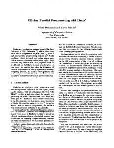
To answer a partial-match query, a hash key is constructed from the query, using the same hash functions which are used to store the data. The hash function for each attribute value speci ed by the query is applied to the value of the attribute, forming a bit string for the attribute. The hash key is formed from the choice vector and the bits strings. The bits in the choice vector of attributes which were not speci ed in the query are not set in the hash key. All the blocks in the data le which match the hash key are retrieved and searched for matching records. If a bit is not set in the hash key, blocks with either value for that bit in their address must be retrieved. We use an \*" to mark the place of the each bit in the 6

Hash key 1**0*01 1000001 1000101 1010001 1010101 Blocks retrieved 1100001 1100101 1110001 1110101

Figure 2.1: Blocks matching the hash key 1**0*01. hash key which is not set. For example, consider the choice vector in the previous section. Assume that a query speci es values for attributes 1, 2 and 3, but not attribute 4. Assume that the values of the attributes speci ed in the query result in the following bit strings:

h1 (A1 ) = 0100110010001; h2 (A2 ) = 1000101011110; h3 (A3 ) = 1110010001100: Combining these bit strings, as speci ed by the choice vector, results in the hash key 1**0*01. The resulting eight blocks retrieved to answer the query are shown in Figure 2.1. The order of the bits in the choice vector can have an impact on the performance of the retrieval algorithm. For example, two consecutive disk blocks can be retrieved faster than two non-consecutive disk blocks because no seeking is required to locate the second block once the rst has been read. Faloutsos [17] suggested using Gray codes to map the hash keys to disk blocks so that records with similar hash keys are clustered together. Any two block addresses which only dier in precisely one of the last two bit positions will be located in consecutive blocks. This results in better retrieval performance. Without additional information to aid in determining what the composition of the choice vector should be, the choice vector for a relation usually consists of an equal number of bits from each attribute. By using additional information, such as the probability of each attribute being accessed and the cost of this access, better 7

sp

0

2d ? 1

2d ? 1

fs

2d+1 ? 1

Figure 2.2: A linear hash le organisation. choice vectors can be built. This is our aim in Chapters 3, 4 and 6. Aho and Ullman [2] described how to determine the optimal number of bits to take from the bit string of each attribute to make up the choice vector for partialmatch retrieval. We refer to this as the optimal bit allocation. Their method assumes that the probability of each attribute appearing in a query is speci ed, and that the probabilities are independent of each other. Moran [54] showed that for the general problem, when the probability of an attribute appearing in a query is not independent of the other attributes, nding the optimal bit allocation is NP-hard. Lloyd [48] presented an ecient heuristic algorithm for nding a good solution to this general problem.

2.1.2 Dynamic les using linear hashing with partial expansions In the previous subsection, we assumed that the size of a hash le was of the form 2d , where d is a non-negative integer. If this is maintained, the le size must double to increase the size of a le. Instead of increasing the le size in one step from 2d to 2d+1 , Litwin proposed the linear hash le [46], in which the size of the le increases one block at a time. Increasing the le size directly from 2d to 2d+1 is an expensive operation because all the records in the le must be examined to determine their new location. It also wastes space, because the storage utilisation, that is, the proportion of the le which contains records, halves in a single step. By choosing appropriate hash functions and increasing the le size by one block at a time, only the records in one block must be rearranged during any single step. A linear hash le may be increased in size by either a single expansion stage, or by a series of partial expansions, as suggested by Larson [42]. We now describe the process of increasing its size using a single expansion stage. Consider the le represented in Figure 2.2. The current le size is denoted by the point fs, which represents the last block in the le and is at a block between blocks 2d ? 1 and 2d+1 ? 1. The split pointer is indicated by the point sp, and is such that fs = sp + 2d ? 1. It denotes the next block to be split when the le size increases. 8

The blocks in the ranges [0; sp ) and (2d ? 1; fs ] are addressed using the rst d +1 bits of the choice vector. The blocks in the range [sp ; 2d ? 1] are addressed using the rst d bits of the choice vector. To search for a record, an address, a, is calculated using d + 1 bits. If a  fs , the block matching the address can be retrieved. If a > fs , the block matching the address a ? 2d must be retrieved. When the le size is increased, the steps of the following algorithm, which is functionally equivalent to one by Larson [42], are performed: increment fs by one for each record r in the block indicated by sp calculate the hash key k using the rst d + 1 bits of the choice vector add r to the block indicated by k (either block sp or sp + 2d ) increment sp by one if sp = 2d , then increment d by one set sp to zero .

To reduce the le size, the process is performed in reverse: if sp = 0, then decrement d by one set sp to 2d ? 1 else decrement sp by one for each record r in the block indicated by sp + 2d add r to the block indicated by sp decrement fs by one .

In the standard linear hashing scheme, if a block becomes full, additional records which are inserted into the block are stored in an over ow chain. This is a set of blocks associated with a single block in the hash le. They are typically stored as a linked list, with the head of the list being the block in the hash le. If over ow chains are long, the average number of blocks which must be searched to nd a record, the average search length, can be signi cantly greater than the optimal length of one (when there are no over ow blocks). The storage utilisation will also be lower. This is because more blocks are used to store the data than is necessary in the ideal case. Using the method described above to increase the size of the le results in an uneven decrease in the storage utilisation. When a block with no over ow blocks is split, the storage utilisation of the two resulting blocks is half that of the original block. A higher storage utilisation, for a given average search length, can be achieved by using linear hashing with partial expansions. A full expansion increases the size of a le from G
N to G
2N by splitting each of the N blocks into two, a block at a time, in the manner we have just described. By using partial expansions, the le size increases from G
N to (G + 1)
N , to . . . , to (2G ? 1)
N , to G
2N . While this  This notation is explained in Appendix A.

9

N

N

2N

Figure 2.3: Two splits in two partial expansions of a linear le, G = 2. still results in an uneven decrease in the storage utilisation, the dierence is much smaller than that of the scheme described above. During the rst partial expansion, G blocks are split into G +1 blocks by moving some records from each of the G blocks into block G + 1. Records are not moved between the G blocks. During the second partial expansion, G + 1 blocks are split into G + 2 blocks, in the same way as in the rst partial expansion. This is repeated for each of the G partial expansions. During the last partial expansion, 2G ? 1 blocks are split into 2G blocks. The value of N is then set to 2N , so that there are G groups of 2N blocks instead of 2G groups of N blocks, and the process starts again. This was analysed and discussed in more detail by Ramamohanarao and Lloyd [65]. Figure 2.3 contains an example of two splits in two partial expansion steps. In this example G = 2. The rst partial expansion moves some records from two blocks to a third, and the second partial expansion moves some records from three blocks into a fourth. By using linear hashing, the reallocation of records to new blocks is ordered and does not occur all at once. Therefore, the cost of increasing the size of the le is low. In a dynamic environment, the bits from the bit string of each attribute composing the choice vector are usually interleaved so that the degradation in performance as the size of the data le changes is minimised. For example, for a le with four attributes in which d = 12, the choice vector would be more likely to be b11b21 b31 b41 b12 b22 b32 b42 b13 b23 b33 b43 , rather than b11 b12 b13 b14 b21 b22 b23 b24 b31b32 b33 b34 . Lloyd and Ramamohanarao [49] showed how near-optimal choice vectors can be constructed for dynamic les for partial-match retrieval if the probabilities of the partial-match retrieval queries are known. 10

2.1.3 Disadvantages of multi-attribute hashing One of the biggest disadvantages of multi-attribute hashing is that indexing information is wasted if attributes in a choice vector are correlated. This results in an uneven distribution of records in the blocks of the data le. We refer to this as a non-uniform data distribution. In an extreme example, consider attribute A1 to be a simple transformation of attribute A2 . For example, A1 could represent \age", while A2 represents \date of birth". A query on either attribute could be answered using an index on only one of the attributes by applying the transformation for queries involving the attribute which is not indexed. A solution is to take these relationships into account when implementing the hash functions and allocating bits from the hash values of each attribute. Another solution is to use a data structure which has a greater tolerance for correlated attributes, such as the BANG le [20] or multilevel grid le [83]. These data structures are discussed in the next section.

2.2 Multi-attribute hashing and other data structures A choice vector can be viewed as specifying the order in which the n dimensional attribute space of a relation is divided. That is, each bit in the choice vector divides the domain space of one attribute into two parts. Therefore, this scheme can be applied to other multidimensional data structures such as grid les, k-d-trees, BANG les and multilevel grid les. In the following chapters we use multi-attribute hashing as the indexing technique. However, the utility of our techniques are increased if they can be applied to other data structures. The key point is that there must be some way of mapping a multi-attribute hash key, as described by the choice vector, to each data structure. We now outline some of these other data structures, and discuss how the choice vector can be applied in each case.

2.2.1 Linear hashing Linear hashing with partial expansions, as described in Section 2.1.2, is the data structure we use for the purposes of calculating the costs of various operations throughout this thesis. The hash key for a record, whose construction is determined by the choice vector, speci es the address of the block in the data le in which the record is stored. Thus, the blocks to be retrieved are identi ed without accessing the disk.

2.2.1.1 Recursive linear hashing The recursive linear hashing scheme of Ramamohanarao and Sacks-Davis [66] is an alternative approach to the storing of over ow blocks in linear hash les. It can be used with all versions of linear hashing, including linear hashing with partial expansions, providing that several dierent hash functions can be applied to each attribute. 11

Recursive linear hashing does not use over ow blocks. Instead, over ow records are stored in separate linear hash les. We refer to the standard linear hash le as a level one hash le. To insert a record, rst we attempt to store it in the level one hash le using the normal hash function. If the appropriate block is full, we apply the level two hash function to the record, and attempt to store the record in the appropriate block in the level two hash le. If this is full, we try to store it in the level three hash le, and so on. Ramamohanarao and Sacks-Davis presented results which show that when the storage utilisation is 85%, more than three levels are rarely required. Comparing their results with other schemes, they stated that the average successful search length for recursive linear hashing is smaller than for linear hashing which uses over ow blocks. They also showed that when the storage utilisation is 95%, the dierence in average search lengths is much greater. In recursive linear hashing, at a storage utilisation of 95%, the average successful search length is still close to one disk access. Recursive linear hashing is simply a dierent method of storing over ow records in linear hash les. Therefore, the relationship between the choice vector and the primary data structure does not change.

2.2.2 Other hashing schemes There are a numerous other hashing schemes which can be substituted for linear hashing in the following chapters. Some will require minor modi cations to the cost functions. We now outline some of these schemes.

2.2.2.1 Extendible hashing Extendible hashing, introduced by Fagin et al. [16], is a representative example of a set of hashing schemes which use a directory. A directory consists of a set of entries. Each directory entry has an associated hash key pre x and contains a pointer to a data (leaf) block. Other hashing schemes of this type include expandable hashing [37], dynamic hashing [41], and virtual hashing [45]. Figure 2.4 contains an example of the organisation of a le indexed using extendible hashing. It is taken from an example by Fagin et al. [16]. The depth of a leaf block is de ned to be the minimum number of bits in the hash key required to uniquely identify the block. The depth of the directory is the maximum depth amongst all the leaf blocks. In Figure 2.4, the depth of the directory, block B , and block C is three, the depth of block A is two, and the depth of block D is one. To insert a record, a hash key for the record is generated. The rst d bits of this hash key, where d is the depth of the directory, are used to identify the appropriate directory entry. The pointer associated with this record is retrieved, and the record is inserted into the leaf block that the pointer refers to. To search for a record the same procedure is followed. For example, assume we wish to search for a record with the hash key 101011 using the data structure in Figure 2.4. The rst three bits are 101, so the fth directory entry is retrieved. This points to block D, so the record we wish to retrieve is located in block D. 12

Directory

Leaf Blocks

000 001 010 011 100 101 110 111

A

h() = 00




B

h() = 010




C

h() = 011




D

h() = 1




Figure 2.4: Example le organisation of extendible hashing. Extendible hashing does not use over ow chains. If the leaf block in which a record is being inserted is full, it must be split. When a leaf block splits, its depth increases by one. This may result in the directory having to increase in size to the new depth. For example, in Figure 2.4, if leaf block A lls, it is split into two blocks, both of which are now of depth three. The records from block A with the hash key pre x 000 will remain in the old block, while the records with the hash key pre x 001 will be placed into the new block. The directory entry for the hash key pre x 001 is then updated to point to the new block. If leaf block D lls, it is split into two, both of which are now of depth two. The records with the hash key pre x 10 will remain in the old block, while the records with the hash key pre x 11 will be placed into the new block. The directory entries for the hash key pre xes 110 and 111 must both be updated to point to the new block. If leaf block B lls, it is also split into two, both of which are now of depth four. The records with the hash key pre x 0010 will remain in the old block, while the records with the hash key pre x 0011 will be placed into the new block. The directory does not contain distinct entries for these two blocks, it is of depth three. Therefore, the directory must double in size, to depth four. Each of the directory entries 0000 to 1111 must be updated to point to the correct leaf blocks. Fagin et al. stated that order preserving hash functions can be used much more easily with this data structure compared with other hashing schemes. The problem with order preserving hash functions is that they usually result in an uneven 13

distribution of records across the hash keys. In other hashing schemes, a hash key usually corresponds to a disk block. This results in large numbers of un lled blocks and blocks with long over ow chains. As stated above, extendible hashing does not have over ow chains. Un lled blocks are minimised because a leaf block is only at the same depth, d, as the directory if the number of records in it, and its buddy, is too great to be contained in a block at level d ? 1. Therefore, for an uneven distribution of records, the number of leaf blocks will not be signi cantly greater than for an even distribution of records. However, the directory itself can grow very large if too many records have the same hash key pre x. In the worst case, every n records inserted results in the directory doubling in size, where n is the number of records which can be contained in a block. This will occur when every record has the same hash key pre x. Relating extendible hashing to multi-attribute hashing, we observe that the hash key for a record, constructed using the choice vector, can be interpreted as determining the directory entry which contains the address of the data block in which the record is stored. If the directory is stored on disk, it requires two disk accesses to retrieve one block. Fagin et al. assumed that the directory would be stored in (virtual) memory, so the cost of accessing it is small. For example, let us assume that each pointer to a disk block is four bytes, that each leaf block is pointed to by two entries in the directory (on average), and that a disk block is 8 kbytes. Each disk block can contain 1024 unique leaf block pointers. Therefore, the directory size for an 8 Gbyte data le would be 8 Mbytes. This can easily be contained within the main memory of machines today. For large numbers of large relations the directories would have to be held on disk. However, by implementing a directory cache, the cost of retrieving a disk block from the hash key of a record should be much less than two disk accesses, on average. Lloyd and Ramamohanarao [49] showed that extendible hashing is better than linear hashing for partial-match retrieval, even though extendible hashing has the overhead of directory lookups. This is because extendible hash les do not have over ow blocks, and the number of blocks in the directory which are accessed is small when compared with the number of leaf blocks which must be retrieved to answer a partial-match query.

2.2.2.2 Multilevel order preserving linear hashing Order preserving linear hashing was independently discovered by Burkhard [9], Orenstein, and Ouksel and Scheuermann [62], according to Orenstein [61]. It is implemented by using an order preserving hash function to generate the hash key for records which are then stored in a linear hash le. Instead of taking the d least signi cant bits from the hash key to index a le of size 2d , as is usually done in linear hashing, the d most signi cant bits must be taken. This ensures that the le can expand dynamically while still remaining ordered. The primary problem with order preserving linear hashing occurs when the data is not uniformly distributed. As we discussed above, this is much more likely for order preserving hash functions than normal hash functions. It results in a large number of over ow blocks for some hash keys, and sparsely lled blocks for others. 14

Block 0

1

2

3

4

5

6

7

8

9

N 2

4

2

6

-

5

6

5

-

4

Level 2

4

3

3

-

3

3

3

-

4

Normal Level

4

3

4

Figure 2.5: Example le organisation of multilevel order preserving linear hashing. To overcome these problems, Orenstein proposed multilevel order preserving linear hashing [61]. The problem of long over ow chains was reduced by storing the over ow blocks of each hash key in a B+-tree instead of in a list. The problem of sparse blocks was reduced by assigning dierent levels (depths) to the blocks stored in order preserving linear hash les, and by eliminating sparsely lled blocks. Figure 2.5 shows an example organisation of a multilevel order preserving linear hash le. It is taken from an example by Orenstein [61]. Figure 2.5 contains a multilevel order preserving hash le in which blocks 0, 1, 8 and 9 would normally be at level four, while the other blocks would normally be at level three. Let us assume that the capacity of a block is four records, and a block is sparsely lled if it contains zero or one records. In Figure 2.5, blocks zero, four and eight were sparsely lled, initially containing zero, one and one records, respectively. The sparsely lled block 8 was eliminated by moving all records from it to its buddy block at the previous level, level three. This is block 0 which moved from level four to level three. The sparsely lled block 4 was eliminated by moving all records from it to its buddy block at the previous level, level two. This is also block 0, which moved from level three to level two. As a result of moving the records, the original sparsely lled blocks become free to be used elsewhere, such as an over ow block in a B+-tree. As each block in Figure 2.5 can store a maximum of four records, four blocks, blocks 3, 5, 6 and 7, have additional over ow records stored in separate B+-trees. Relating multilevel order preserving linear hashing to multi-attribute hashing, we observe that a multi-attribute hash key can be used in place of the key of a single attribute, providing it is order preserving. That is, all the hash functions used to compose the multi-attribute hash key must be order preserving, and the most signi cant bits must be taken from the bit strings to form the hash key of a record.

2.2.2.3 Adaptive hashing

The adaptive hashing of Hsiao and Tharp [30] aims to combine the features of order preserving linear hashing and the B+-tree [13]. The hash functions used in adaptive 15

Hash key

0

1

2

3

BP

0

1

3

3

12 14

15 18

DP

3 4

6

7 10

11

21

Figure 2.6: Example le organisation of adaptive hashing. hashing are order preserving. Figure 2.6 shows an example, similar to one by Hsiao and Tharp [30], of the organisation of a le indexed using adaptive hashing. In this case the hash function is bv=8c, where v is the value to be stored in the le. Each leaf block can hold two buckets. In this example, each bucket contains one record. As in extendible hashing, adaptive hashing has a directory and leaf blocks. Unlike extendible hashing, each leaf block has a pointer to its successor, so that a le may be accessed sequentially. The directory consists of two elds for each hash key, a bucket pointer (BP) and a data pointer (DP). Both pointers must be used to determine the rst potential matching record for a hash key. The data pointer refers to the rst block in which a record which matches the hash key may be stored. The bucket pointer records the oset, from the block indicated by the data pointer, of the rst bucket which contains records which do match the hash key. The bucket size can be xed to any value between one record, as in Figure 2.6, and the block size. For example, assume that we wish to nd the value 11. It is located in the rst bucket of the fourth block or, equivalently, the seventh bucket of the le. The hash key is b11=8c = 1. The data pointer for hash key 1 refers to the third block. The bucket pointer for hash key 1 refers to bucket oset 1, that is, the second bucket starting from the third block. This is where we commence our search. We retrieve the third block. The second bucket in this block contains a record with value 10, which does not match. Therefore, we must examine the next bucket. The next bucket is located in the next block, so we now retrieve the fourth block. The next bucket does contain a record with the value we are looking for, so we succeed. This algorithm is linear in the number of buckets which must be examined. Hsiao and Tharp also proposed a binary search algorithm to reduce this cost. 16

When a block over ows during insertion, a new block is created and inserted into the chain of blocks. The directory size is not increased. Note that some bucket pointers in the directory may require updating each time the number of buckets containing records increases, not only when the number of blocks increases. For example, consider the insertion of a record with value 22 into the organisation shown in Figure 2.6. It would be inserted into the second bucket of the seventh block, after value 21. This is the bucket which the block pointer of hash key 3 is referring to. However, b22=8c = 2. Therefore, the bucket pointer of hash key 3 must be incremented to 4. This occurred without increasing the number of blocks. If a record with value 19 is inserted, it would create a new block between the sixth and seventh blocks. In this case, the bucket pointer for hash key 3 would also have to be updated. After a predetermined number of insertions, the directory size is doubled and the blocks are reallocated to directory entries so that there are (approximately) an equal number of blocks between each pair of adjacent directory entries. This may result in large values of BP for some entries, if the data is unevenly distributed. This is why the binary search algorithm is necessary. However, unlike extendible hashing, it does not result in directories which are signi cantly larger than the number of blocks in the le. Relating adaptive hashing to multi-attribute hashing, we observe that a multiattribute hash key can again be used to determine the directory entry for a record. The exact number of disk accesses required to retrieve a record is unknown, because of the bucket pointers. However, the same can be said for linear hashing when over ow blocks are used. For a le with an equal distribution of records to hash keys the cost will be similar to extendible hashing, if the directory is stored on disk, or to linear hashing, if the directory can be maintained in memory.

2.2.2.4 Multidimensional order preserving linear hashing with partial expansions A dynamic hashing scheme introduced by Kriegel and Seeger [39], multidimensional order preserving linear hashing with partial expansions (MOLHPE), combines multidimensional (multi-attribute) hashing, order preserving linear hashing, and linear hashing with partial expansions. By avoiding the directory of data structures such as extendible hashing and the grid le (described below), better retrieval performance than those data structures is ensured for point queries. That is, point queries can be answered in less than two disk accesses on average, providing the data is uniformly distributed. In MOLHPE, each dimension is treated equally. The key space of each dimension is mapped into [0; 1) by an order preserving hash function. Figure 2.7(a) shows an example, by Kriegel and Seeger [39], of a two dimensional data structure and the arrangement of (hashed) key space regions to block addresses. As in linear hashing with partial expansions, the le size is doubled by a series of partial expansions. Only one dimension is expanded at a time. That is, the le size is doubled by splitting in one dimension. Figure 2.7(b) shows the le in Figure 2.7(a) after it has undergone two steps in the rst of the two partial expansions which compose a full expansion. After a full expansion is complete, the le size is doubled 17

K2 1 3 4 1 2 1 4

K2 1

12 14 13 15 2

5

3

3 4 1 2 1 4

7

8 10 9 11 4

0 1 4

1 1 2

6 3 4

1

K1

12 14 13 15 2 17 5 3

8 10 9 11 0 16 4 1 1 1 1 6 3 2

(a)

7 6 3 4

1

K1

(b)

Figure 2.7: Example le organisations of multidimensional order preserving linear hashing with partial expansions. again by splitting in the next dimension. Kriegel and Seeger attempt to overcome the problem of non-uniform data distributions inherent in order preserving hashing schemes by selecting partitioning points based on the distribution of data. Instead of splitting a dimension into two by dividing the key space in half, it is split into two using the half quantile points. These points are stored in memory in a binary search tree. Figure 2.8 shows an example, similar to one by Kriegel and Seeger [39], in which a key space is divided using half quantile points. They claimed that this method guarantees that MOLHPE performs almost as well for non-uniform distributions as it does for uniform distributions. Unfortunately, this is true only if the distribution of data in each dimension is independent of the other dimensions. Therefore, it is not true in general. Relating MOLHPE to multi-attribute hashing, we observe that a choice vector can be used to determine which dimension to split on at each stage, rather than splitting each dimension in turn. Similarly, the bits of a given attribute within a multi-attribute hash key can be used to indicate where in the MOLHPE key space an attribute value lies.

2.2.3 Grid le The grid le of Nievergelt et al. [57] is a multikey data structure which is general enough to encompass a number of dierent implementation strategies. Like the extendible hash le, it is composed of a (multidimensional) directory and data blocks. Several entries in the directory may point to the same data block. In the general 18

K2 y3=4 y1=2 y1=4 x1=4 x1=2 x3=4

K1

Figure 2.8: Example le organisation of multidimensional order preserving linear hashing with partial expansions using quantile splitting. form, it also includes a list of split points for each dimension. That is, a list of points at which the data space is divided into two. These lists are held in main memory. Accessing a record requires two disk accesses, one to the directory and one to the relevant data block. The original grid le scheme does not specify a splitting or merging policy, or how the grid directory should be implemented. These are left to the implementor. However, Nievergelt et al. examined these issues and recommended that the splitting policy should be such that a block is always divided into two blocks during splitting. They reasoned that splitting a block into more than two blocks results in a signi cantly lower average block occupancy. The choice of dimension and location within the dimension to split on were not speci ed. They noted that one policy is to choose the dimension according to a xed schedule, such as cyclically. The location of the split could be the midpoint of the interval being split, but it need not be. Nievergelt et al. compared the buddy and neighbour systems for block merging. In the buddy system, a block can only merge with one adjacent, equal-sized buddy in each dimension. In the neighbour system, a block can merge with either of its two adjacent neighbours in each dimension, providing the resulting region is convex. Every buddy is a neighbour, but not every neighbour is a buddy. Two blocks are available to be merged if the number of records in the two blocks can be contained within a single block. The neighbour system results in a higher storage utilisation because a neighbour is more likely to be available for merging than a buddy. The grid directory may be implemented in many ways, from lists of lists to a multidimensional array. Nievergelt et al. favoured the multidimensional array for space eciency. In this implementation, each time a dimension is split, the directory size doubles because the space covered by each directory entry is divided 19

into two. However, the number of data blocks is only increased by one. Therefore, many of the data blocks are pointed to by multiple directory entries. The periodic doubling of the directory size is a disadvantage of this implementation the grid le. However, Nievergelt et al. claim that this is likely to be rare occurrence unless the data distribution is highly non-uniform, such as when attributes are highly correlated. In the worst case, the directory can grow exponentially. When others have discussed the grid le, it has generally been assumed that the directory is stored as a multidimensional array, that dimensions are always split into two at the midpoint of the range, and dimensions are typically chosen cyclically. It is easy to see how aspects of multi-attribute hashing can be translated to this storage method. The bits provided by each attribute in the choice vector can be used to determine which point in the domain of each dimension that the multiattribute hash key represents. The order of the bits in the choice vector can be used to determine which dimension to split on. The multilevel grid le is also based on this approach.

2.2.4 Multilevel grid le The multilevel grid le of Whang and Krishnamurthy [83] was designed to overcome the problem of the grid le directory size when it is implemented as a multidimensional array. It achieves this by rede ning how a grid entry is calculated and by making the directory a tree. Figure 2.9, by Whang and Krishnamurthy [83], shows a partitioned data space in which the dashed boxes represent data blocks. Below it there is a two level directory for the data space. The design of the multilevel grid le diers in some details from the grid le. Instead of splitting a directory based on attribute values, each dimension has an associated hash function which returns a bit string. A dimension is then split using the bits of its hash function. The directory entries contain bit string pre xes and their associated pointers. This is shown in Figure 2.9. If range queries are to be performed eciently, order preserving hash functions must be used. To perform a query, the directory tree is traversed to nd the appropriate data blocks, which are then retrieved. For example, consider the partial-match query which does not specify a value for the rst attribute, but does for the second attribute, against the data structure shown in Figure 2.9. Assume that the value of the second attribute returned by the hash function has a bit string pre x of 01. Thus, we must search for blocks with pre xes ({,01). We start at the top of the multilevel grid le directory, and nd that the rst, third and fourth entries match our query. Therefore, three entries at the second level must be searched. In the rst of the three, the third and fourth entries match our query. We must retrieve their associated data blocks, and search them for answers to our query. In the second of the second level directory entries we must examine, the third directory entry, both the second and third entries match our query, so their data blocks must be retrieved and searched. In the third second level directory entry we must examine, the fourth directory entry, the rst two entries match our query, so both their data blocks must be retrieved and searched for matching entries. Thus, we must search six data blocks for potentially matching records. Grid regions with no associated data blocks do not appear in the directory hi20

11 10 01 00 000

001

010

011

100

101

110

111

000,00 001,00 00 ,01 01 ,{ 0 ,{ 1 ,1 10,0 11,0

1 ,10 1 ,11 Data blocks 100,00 100,01 101,0 110,01 111,01 11 ,00

Figure 2.9: Example le organisation of a multilevel grid le.

21

erarchy. For example, in Figure 2.9, the region with the pre xes (00,1) does not have an associated data block. Therefore, it does not appear in the second level of the index. Grid regions appear only once at any directory level. For example, the region with the bit string pre xes (01,{) has only one data block. Consequently, it has only one entry in the second directory level, the last entry of the rst directory block. These two features ensure that the directory will grow at the same rate as the data, even for non-uniform data distributions. Therefore, the multilevel grid le does not have the same worst case performance as the standard grid le, in which the directory size can double each time a new data block is required. It is clear that the concept of using a choice vector to determine where to store a record can be applied to the multilevel grid le as easily as multi-attribute hashing. To use a choice vector, we assume that hash functions must be associated with each attribute, and that the choice vector speci es the order in which the dimensions should be split. Data stored in a multi-attribute hash le can be stored in a multilevel grid le, by using the choice vector to determine the appropriate grid region. The cost of each operation would change because of the need to consult the multilevel directory. However, the size of the multilevel directory is much smaller than directory of the grid le. Fewer disk accesses would typically be necessary with the multilevel grid le for queries other than point queries, and many of the upper directory levels would be able to be contained within memory.

2.2.5 BANG le The BANG le of Freeston [20, 21] is a multilevel, multidimensional le structure in the same class as the grid le and multilevel grid le. Unlike those two structures, in which the data blocks spanned disjoint regions, the data blocks in the BANG le can span nested regions. Figure 2.10 shows an example of two dierent BANG le structures with blocks of dierent capacities. The solid boxes denote a data block, the circles denote records. The rst organisation contains four blocks, each containing two records; the second organisation contains three blocks, each containing two or three records. Both organisations are balanced. The nesting of blocks enables the records to be distributed in a much more balanced way, even for highly non-uniform data distributions. A nested region need not be convex, providing that it is completely contained within its enclosing block. Nesting also permits the redistribution of data by changing the regions the blocks cover if the data distribution changes. Theoretically, a block may even be composed of disjoint regions, providing its enclosing block spans both regions. Like the multilevel grid le, which postdates the BANG le, regions are denoted by bit strings. While the directory blocks are stored as a tree, the directory entries are stored as a list within each block, with the smallest region rst. When retrieving records, the search algorithm must start at the beginning of the block, that is, at the smallest possible region. For example, consider the rst le organisation shown in Figure 2.10. The directory would contain encodings for four regions and their associated block pointers. The rst region is (2,2), the second region is (3,2), the third region is (2,2) to (3,3) and the last region is (0,0) to (3,3). Consider a query searching for the record located in the region (2,3). Each region listed in the directory will be compared with 22

3 2 1 0 0

1

2

3

Figure 2.10: Example le organisations of a BANG le. the region in which the record is located. The rst two will fail to match. The third does cover the region the query was asking, so the data block for the third region must be retrieved to nd the record. The outermost region always encompasses the entire data space, so the record will always be found in precisely one block. The order in which dimensions are split is often cyclic, but need not be. A choice vector can be used to determine which grid region a record should be contained in and in which order the dimensions should be split.

2.2.6 Multidimensional binary search tree The multidimensional binary search tree (k-d-tree) was introduced by Bentley [3]. He later summarised further research into the data structure by himself and others, and placed the research in the context of database management systems [4]. The k-d-tree is a generalisation of the binary search tree, extended to k dimensions. It has two forms, homogeneous and non-homogeneous. In the homogeneous form, a single record is stored in each node of the tree. In the non-homogeneous form, there are two types of nodes, internal nodes and leaf nodes. The internal nodes only contain key values, all the records are stored in the leaf nodes. Homogeneous k-d-trees are usually used when all the data is stored in main memory, non-homogeneous k-d-trees are used when the records are stored on disk. If the records are stored on disk, the leaf nodes typically correspond to a disk block and contain a number of records. Conceptually, a node in a k-d-tree consists of k keys, a left subtree pointer, a right subtree pointer, a discriminator and data elds. The discriminator denotes which of the k keys should be used to determine whether to examine the left or right subtree for a given query. The records in the left subtree all have a value for the key indicated by the 23

discriminator which is less than that of the current node. The records in the right subtree all have a value for the key indicated by the discriminator which is greater than that of the current node. The location of records with values equal to the key depends on the type of k-d-tree. In a non-homogeneous k-d-tree, records with values equal to the key are always placed in the right subtree. In a homogeneous k-d-tree, if a record is being inserted which has the same value for the discriminating key, then the next of the k keys is examined to determine which subtree to place the new record in. In some implementations, some elds are not included in a node. For example, in a non-homogeneous k-d-tree in which the keys are used cyclically, level i uses key (i mod k) and does not require k ? 1 of the keys, the discriminator or the data elds. If a multi-attribute bit string and choice vector is used, this may be further reduced to just the left and right subtree pointers for each node. In the original paper [3], Bentley suggested that each of the k keys should be used in turn as the discriminator. In a subsequent paper [4], he acknowledges that one may do better by choosing a discriminator which is often speci ed in queries. The choice vector can do just that. For many large data les, it is unlikely that even a non-homogeneous k-d-tree index will be able to be stored in memory for every data le. Therefore, accessing a single record requires two disk accesses, one to the index and one to the data block. However, if many data blocks will be retrieved with similar keys, the relative overhead of accessing the index will decrease dramatically.

2.2.7 Other data structures There have been many other data structures proposed which are similar to, or are variations on, the data structures described above to which we can apply our techniques. They can be categorised as spatial data structures which are able to eciently store and access point data, in addition to the region data and queries with which they are primarily concerned. Samet [70] discusses more of these. Most, if not all, of these structures can use the choice vector of multi-attribute hashing to determine where a record should be placed, and which dimension to split on when subdivision of the dimension space is required.

2.3 Join algorithms The analysis and implementation of the join operation has been an active area of research. It was recently surveyed by Mishra and Eich [53]. There are three main types of join algorithm which are used when no indexes are available: nested loop, sort-merge and hash join. While often only one of the sort-merge and hash join algorithms is implemented in a database system, Graefe et al. [26] demonstrated that each performs better than the other under known circumstances and argued that each should be available in a database system. Variations of all three algorithms are analysed in subsequent chapters. This section contains an overview of each algorithm, providing the foundation upon which our variations are based. 24

We de ne a buer to be a set of related blocks in main memory. They need not be contiguous. The amount of main memory available to be used as buers is considered to be a buer of size B blocks. The size of a buer, in blocks, is given in the form Bx . When there can be no confusion, we also use this size as a label for the buer. The notation used in this thesis appears in Appendix A.

2.3.1 Nested loop The nested loop algorithm is the simplest of the join algorithms. It works in the following way. For each record in one relation, the outer relation, the other relation, the inner relation, is scanned and the pairs of records satisfying the join condition are used to produce the result records. The outer relation is typically the smaller of the two relations. In practice, more than one record of the outer relation is read before the inner relation is scanned. For example, Blasgen and Eswaran [7] held as many records of the outer relation in memory as possible and read one record at a time from the inner relation. A similar algorithm has been suggested on the disk block level. That is, B ? 2 blocks of the outer relation are read at a time, and the inner relation is scanned one block at a time. One block is reserved for the result records. This algorithm is often called the nested block algorithm. We use the term nested loop join to encompass all of these algorithms. Its operation may be described as follows: while there are unread records in the outer relation read records from the outer relation into buer B1 seek to the beginning of the inner relation while there are unread records in the inner relation read records from the inner relation into buer B2 inner loop for each record r1 in B1 for each record r2 in B2 if r1 and r2 satisfy the join condition place the result record in buer BR if the buer BR is full, write it to the result relation

In the above algorithm, we assume, without loss of generality, that the rst relation is the outer relation. Figure 2.11 shows the arrangement of the buers in memory for the nested loop join algorithm. The size of the buer for the outer relation, B1 , will usually be larger than that of the inner relation, B2 , unless the outer relation is very small. There is no bene t in having the size of a buer being larger than the size of its associated relation. Several optimisations can be applied to the above algorithm. Two are the use of a hash table, and rocking. Instead of comparing every record in B1 with every record in B2 , the records in B1 can be inserted into a hash table using the join attributes to form a hash key. The records in B2 are then used to probe the hash 25

Main memory, B

B1

B2

BR

Figure 2.11: Buer arrangement for the nested loop join algorithm. table, searching for records to join with. This signi cantly reduces the number of comparisons required. Rocking, suggested by Kim [34], is used when the outer relation is larger than its memory buer, B1 . On the rst pass through the inner relation, the inner relation is read from disk. On subsequent passes, part of the inner relation will already be in memory, from the previous pass. This part need not be reread from disk. The name, rocking, derives from the observation that one implementation of this is to read the inner relation forwards and backwards on alternate passes. Thus, the beginning and end of the relation is only read from disk on alternate passes. In most operating systems it is much more ecient to read a le forwards than backwards. Under these circumstances, a better implementation of rocking is to read the le in a circular manner. Each pass should start by processing the records already in memory. It should then start reading from the end of the last part of the le read during the previous pass and read to the end of the le. It should then go back to the start of the le and read to the start of the rst block of the le which was in memory at the beginning of the pass. The same number of blocks are read as in Kim's scheme, but the total time taken to read it will be shorter because the le is always read in the forwards direction.

2.3.2 Sort-merge The sort-merge join works in two phases, a sorting phase and a merging phase. In the sorting phase, each relation is sorted using the join attributes. In the merging phase, each sorted relation is scanned in parallel, and records with matching join attributes are joined. By rst sorting both relations, the merging phase is performed in linear time in the size of the relations. The sort-merge algorithm presented below is similar to the version used in the Aditi deductive database system [80], and is more general than that described above. During the sorting phase, the relations are not fully sorted. Instead, each relation is divided into partitions which are sorted. The size of the partitions is the size of the memory buer, B . During the merging phase, the sorted partitions of each relation are merged using a multiway merge and then the records from each relation are joined. These two operations are pipelined. 26

The following description assumes that the total number of partitions formed from both relations is such that they may be merged in memory in one pass. If this is not the case, the sorting phase must be extended to merge some of the sorted partitions, reducing the number of partitions to be merged so that they can be merged in memory in one pass. The operation of the sort-merge algorithm may be described as follows: sorting phase while there are unread blocks in the rst relation read records from the rst relation into buer B sort the records in buer B write the records in buer B out to a new partition while there are unread blocks in the second relation read records from the second relation into buer B sort the records in buer B write the records in buer B out to a new partition

merging phase for each partition, i, of the rst relation read records into the ith buer of size B1 form a priority queue from the rst record in each of the buers of size B1 for each partition, i, of the second relation read records into the ith buer of size B2 form a priority queue from the rst record in each of the buers of size B2 while there are unmerged records merge and join records from the two priority queues replace the merged records in the priority queues with their successors from their . . . original buers if the ith buer of size B1 is empty . . . and there are unread records in the ith partition of the rst relation read records from partition i of the rst relation into the ith B1 buer add the rst record just read to the rst priority queue if the ith buer of size B2 is empty . . . and there are unread records in the ith partition of the second relation read records from partition i of the second relation into the ith B2 buer add the rst record just read to the second priority queue

We assume that the merging phase will produce the correct output when successive records from one partition have the same values for the join attributes. If the size of the rst and second relations are V1 and V2 blocks respectively, there will be dV1 =B e partitions of the rst relation and dV2 =B e partitions of the second relation. During the merging phase, the available memory is divided into buers for each partition of each relation, as shown in Figure 2.12. Note that the buers of size B1 and B2 need not all be the same size. Replacement selection, as described by Knuth [38], can also be used to generate the initial sorted partitions. This results in an expected partition size of 2B , so there will be only dV1 =(2B )e and dV2 =(2B )e partitions generated from each relation, 27

Main memory, B

B1




dV1 =B eB1

B1






B2

B2

BR

dV2 =B eB2

Figure 2.12: Buer arrangement for the merging phase of the sort-merge join algorithm. respectively. However, the relations must be read using many more read operations (and hence seeks) than the scheme described above, which lls the buer on each read.

2.3.3 Hash joins

Hash join algorithms take advantage of the fact that the nested loop algorithm only requires a single scan of the input relations if one of the two relations can be completely contained in memory. They aim to partition the relations so that this is possible. Here we describe the original partitioning hash join algorithm, the GRACE hash join, and an important variation, the hybrid hash join. Both algorithms work in two phases.

2.3.3.1 GRACE hash join During the rst phase of the GRACE hash join algorithm [36], each record of the input relations is read and a hash function is applied to the join attributes of the records. The result of applying the hash function is used to form a hash key for each record. The hash key is used to determine which output partition each record is placed in. The input relations are partitioned into pairs of partitions (one per relation). If the smaller partition in each pair of partitions is larger than main memory the pair of partitions are themselves partitioned into pairs of smaller partitions. This process continues until at least one partition in each pair can be contained in memory. The same hash function must be used to partition each relation, producing the same number of partitions, P , from each relation. If two records must be joined they will have the same hash key, and, therefore, will be in the same partition of each relation. The buer arrangement during the partitioning phase of the GRACE hash join algorithm is shown in Figure 2.13. In it, the size of the input buer is denoted by 28

Main memory, B

BI






BP

BP

PBP Figure 2.13: Buer arrangement for the partitioning phase of the GRACE hash join algorithm.

BI , and there are P output partition buers, each of size BP .

The algorithm to partition a single relation may be described as follows:

partition while there are unread blocks in the relation read records from the relation into buer BI for each record in buer BI form a hash key from the join attributes of the record use the hash key to select an output buer BP move the record to BP if BP is full, write it to its output partition on disk

In the second phase of the GRACE hash join algorithm, the nested loop algorithm is applied to each pair of partitions. In each case, the outer relation is read and its records inserted into a hash table. Then the inner relation is scanned and the hash table is probed to join the records. The buer arrangement for this phase is the same as that given in Figure 2.11. The GRACE hash join algorithm may be described as follows: partitioning phase while there are pairs of partitions which are both larger than main memory partition the relevant partitions of the rst relation into P partitions partition the relevant partitions of the second relation into P partitions partition joining phase for each partition of the rst relation use nested loop to join it with the matching partition of the second relation

The number of partitions created during each partitioning pass, P , must be the same for each relation. However, P may vary between partitioning passes. 29

Main memory, B

BI

BH

BP






BP

BR

PBP Figure 2.14: Buer arrangement during partitioning in the hybrid hash algorithm.

2.3.3.2 Hybrid hash join The hybrid hash join algorithm of DeWitt et al. [15] is similar to the GRACE hash join algorithm. The primary dierences are that it assumes that there is sucient memory so that only one partitioning pass is required, and during the partitioning pass an area of memory is reserved to perform joins in. Instead of hashing each record into one of P partitions during the partitioning phase, each record is hashed into one of P + 1 partitions. During the partitioning of the rst relation, records which hash into the extra partition are not written to disk but are stored in a hash table, BH , in memory. When the second relation is partitioned, records which hash into the extra partition are joined with the records of the rst relation which are stored in the hash table by probing the hash table, as in the nested loop algorithm. The amount of memory reserved for the hash table need not be the same as the expected size of the other partitions, providing that the extra partition does not over ow during the partitioning of the rst relation. In the algorithm given below, we assume that the hash table does not over ow. We discuss algorithms which gracefully handle hash table over ow in the next subsection. The buer arrangement during the partitioning phase of the hybrid hash join algorithm is shown in Figure 2.14. Note that there must also be a result buer, BR , to hold the result of joins using the hash table during the partitioning phase. The second phase of the hybrid hash join is exactly the same as that of the GRACE hash join. The hybrid hash join algorithm may be described as follows: partitioning phase while there are unread blocks in the rst relation read records from the rst relation into buer BI for each record in buer BI form a hash key from the join attributes of the record use the hash key to select an output buer BP or the hash table BH move the record to BP or BH if BP is full, write it to the output partition on disk

30

while there are unread blocks in the second relation read records from the second relation into buer BI for each record in buer BI form a hash key from the join attributes of the record use the hash key to select an output buer BP or the hash table BH if BP was selected move the record to BP if BP is full, write it to the output partition on disk if BH was selected join with matching records in the hash table, moving the results to BR if the buer BR is full, write it to the result relation partition joining phase for each partition of the rst relation use nested loop to join it with the matching partition of the second relation

2.3.3.3 Other hash join variations A number of other hash join algorithms have been proposed. Most of these are extensions to the hybrid hash algorithm, and attempt to relax the assumptions made in its design. Their primary aim has been to overcome the problems of an uneven distribution of data which can result in large dierences in the sizes of the partitions of a relation. The following chapters primarily use the GRACE or hybrid hash algorithms as examples of hash join algorithms. However, the following join algorithms could also be used. Nakayama et al. [56] proposed using a dynamic destaging strategy during the partitioning phase. It creates many buckets into which the input relations are partitioned. The number of buckets is typically much greater than P . All buckets initially start as internal, that is, they are held in a hash table in memory, as in the hybrid hash algorithm. However, they may migrate to being external, that is, stored on disk. Once all the blocks in memory are allocated for use and more are required, the largest bucket is changed to be external and all its hash table blocks are written to disk. The bucket retains one block in main memory to be used as its output buer. The other blocks it used are now available to be used by the remaining internal buckets. This process continues throughout the partitioning phase: whenever all the memory blocks are used, the largest internal bucket is changed to be external. After the partitioning phase is complete, the buckets are grouped into partitions. The partition joining phase now starts. It is the same as in the GRACE and hybrid hash algorithms. The only advantage in grouping buckets into partitions is that the number of times that the hash table in memory must be initialised is reduced. No comparison was made between the amount of time saved using this method and the amount of time taken to determine a good grouping. Zeller and Gray [85] described an adaptive hash join. It is a variation of the hybrid hash join which allows the amount of memory available to perform the join in to uctuate during the execution of the join. It does this by using many buckets for each relation and dynamically changing the number of the buckets held in a hash 31

table in memory. Unlike the scheme of Nakayama et al., the internal buckets are initially grouped into partitions. This grouping of buckets to partitions can change if a partition becomes too large, that is, if the outer partition becomes larger than the expected size of main memory during the partition joining phase. Initially, when all the memory is used during partitioning but no partition is larger than the amount of memory, a bucket will move from being internal to external. Later, when a partition becomes too large, the partition is split and its buckets are divided between the two new partitions. During the partition joining phase, the part of the original partition already written to disk will have to be read by both new partitions. This scheme allows the number of buckets held in memory to change dynamically, if the amount of memory available to perform the join changes. Partitions can be split by dividing the buckets between new partitions if the amount of memory available decreases, and partitions can be joined if the amount of memory available increases. Pang et al. [64] introduced a class of partially preemptible hash joins. It is more general than the scheme of Zeller and Gray. Not only does it turn internal partitions into external partitions when the amount of available memory decreases, but it turns external partitions into internal partitions if more memory becomes available. The partially preemptible hash joins also permit output buer blocks to be allocated priorities, so that when more blocks are required for internal partitions they are taken from the output partitions of particular external partitions rst. The authors report that this class of join algorithm has superior performance to the other four algorithms discussed above when the amount of memory available uctuates throughout the execution of the join.

2.4 Combinatorial optimisation techniques Finding the optimal solution for many of the problems we will discuss is NP-hard. Our aim was to nd good solutions in a reasonable amount of time. It was not to nd the fastest possible algorithm in each case, which would require domain speci c knowledge for each problem. To attempt to nd good solutions we tested both heuristic techniques and combinatorial optimisation algorithms. In this section, we introduce the combinatorial optimisation techniques we used.

2.4.1 The optimisation problem

Our optimisation problems can all be described in the following way. Consider a set, d~, of n non-negative integers, di , upon which we de ne a cost function, f . C = f (d~) d~ = fd1 ; d2 ; : : : ; dn g: Our aim is to nd d~min , such that f (d~min )  f (d~), for all d~. The constraint n X i=1

di = d 32

must be satis ed. Relating this to multi-attribute hashing, di is the number of bits allocated to the ith attribute, d~ is a bit allocation, and d~min is the optimal bit allocation.

2.4.2 Minimal marginal increase

Minimal marginal increase (MMI) is a greedy algorithm which works incrementally. It commences with di = 0, for each di . Therefore, d = 0. It increments d, so that d = 1. It then determines d~min for d = 1. It does this by incrementing each di by one in turn, while leaving the other di 's at zero, and calculating the value of the cost function. The d~ which resulted in the smallest value of the cost function is d~min for d = 1. This is chosen to be permanent. We say that the di which is incremented as a result of this is allocated a value. The set d~min for d = 2 is then determined. This is done by starting with d~min for d = 1, and incrementing each di by one, in turn, and calculating the value of the cost function. The smallest value of the cost function determines which of the n sets is d~min for d = 2. This process is repeated until d reaches the desired value. The minimal marginal increase algorithm may be described as follows: for each i from 1 to n set di to be 0 for each d from 1 to the nal d set the best cost, c0 , to be 1 for each i from 1 to n increment di by 1 calculate the cost, c, to be f (d~) if c is less than the best cost, c0 set the best cost, c0 , to be c set d~min for the current d to be d~ decrement di by 1 set d~ to be d~min

According to Lloyd and Ramamohanarao [49], this algorithm usually nds the optimal bit allocation for a relation when considering partial-match queries. They reported that when it does not nd the optimal bit allocation, the average query cost of the bit allocation is, at most, a few percent higher than that given by the optimal bit allocation. Minimal marginal increase sets d~min at level d prior to searching at level d + 1 and never removes an allocated value from a di . Therefore, it is possible that it will not nd the optimal d~. For example, assume that the optimal d~ for n = 3 is f3, 8, 5g (d1 = 3, d2 = 8, d3 = 5). Also assume that the cost of f4, 4, 2g is lower than the cost of f3, 5, 2g and f3, 4, 3g. If we reach f3, 4, 2g, then the optimal d~ can never be found. The set f4, 4, 2g will be chosen in preference to either of the other two sets, and the fourth value allocated to d1 will never be removed.

2.4.2.1 Minimal marginal increase and multi-attribute hashing

One of the constraints for the data structures described in the previous sections to be dynamic is that the choice vector of length d must be the rst d bits in the choice 33

vector of length d + 1. If this is not the case, the cost of reorganising the data les is not linear in the number of new blocks added. By starting with zero bits allocated to each attribute, minimal marginal increase produces the best incremental bit allocation for each possible le size from 1 to 2d . If the size of the data le increases, then the bit allocation for the new size can be determined by calculating the next bit, using the existing bit allocation as the starting point. Similarly, if the data le decreases in size, the bit allocation to use will simply be the rst d ? 1 bits allocated. It is very easy to modify the minimal marginal increase algorithm so that an attribute is not allocated more than its constraining number of bits.

2.4.3 Simulated annealing Simulated annealing (SA) [1] is a class of optimisation algorithms based on Monte Carlo techniques. The algorithm we used is substantially the same as that used by Ramamohanarao et al. [67]. Our simulated annealing algorithm implementation performs a number of trials, T , and returns the d~ with the smallest value for the cost function from amongst the trials. In each trial, a random d~ is generated (the trial seed), and the value of the cost function is calculated. We then perform sequences of perturbing operations, starting with this initial d~. The length of each sequence, P , is called the Markov chain length. We refer to the sequence as a chain of perturbing operations. A set, d~, is perturbed by decrementing a number from one randomly selected di and incrementing, by the same number, a dierent randomly selected di . The value of the cost function for this d~ is then calculated. If this value is less than the value of the cost function for the previous d~, or a randomly generated probability is less than the acceptance probability , this d~ is used as the basis for the next iteration, otherwise the previous d~ is used. The number of chains is determined by the cost obtained at the end of each chain. If the cost does not alter for a xed number of chains, F , the trial terminates with the last cost as the nal cost of the trial. In all our results, F was set to 100. This was the value used by Ramamohanarao et al. The acceptance probability can be written in the form Pr = Q(1T ) e?
C=T where T is the temperature, Q(T ) is a normalisation constant which depends on T , and
C is the dierence between the current and best trial costs. As the number (not length) of the current chain increases, the temperature is reduced according to a cooling schedule. The eect of the cooling schedule is that the simulated annealing algorithm is more likely to accept a d~ with a higher cost than the current cost in early trials than in later trials. It is also more likely to accept costs which are only slightly worse that the best trial cost than costs which are signi cantly worse. This is done so that better sets may be found which can only be reached from the initial seed by passing through a worse d~. 34

Our simulated annealing algorithm may be described as follows:

set the best trial cost, tc, to be 1 for each of T trials generate a random d~ set the best chain cost, bcc, to be 1 set the number of chains at the current bcc, bcn, to be 0 set the chain number, cn, to be 0 while bcn is less than F set the chain cost, cc, to be 1 increment cn by 1 for each of the P perturbing operations in the chain randomly select two values, di and dj , in d~ randomly select the number, b, to perturb by such that di ? b  0 decrement di by b increment dj by b calculate the cost, c, of d~ if c is greater than cc and the temperature comparison function is false increment di by b decrement dj by b else set cc to be c if cc is less than bcc set bcc to be cc set bcn to be 0 else increment bcn by 1 if bcc is less than tc set tc to be bcc save the best d~

temperature comparison function return exp((cc ? c)=(Ccool  (Cctrl )cn )) Our cooling and control constants, Ccool and Cctrl , determine the rate of cooling at which poorer values for the cost function are accepted. The values we typically used for these two variables were 1 and 0.95, respectively. These values were chosen to ensure that the running time of the simulated annealing algorithm was acceptable for our larger problems, and are in the range suggested by Aarts and Korst [1]. When used to search for the optimal bit allocation, the simulated annealing algorithm can be modi ed to ensure that an attribute is not allocated more than its constraining number of bits. While simulated annealing is not ideal for all optimisation applications, as shown by Nahar et al. [55], in the past it has proved to be a useful means of obtaining nearoptimal indexes in applications of the type we will consider [67]. It has also been suggested for use as a basis for other techniques in query optimisation. Some of these include the join query optimisation of Swami [76], the two phase optimisation of Ioannidis and Kang [33], and optimisation in parallel execution spaces by

35

Lanzelotte et al. [40]. Note that the \toured" simulated annealing of Lanzelotte et al. is simply simulated annealing with multiple trials using a dierent, application speci c, method of determining the seed for each trial.

2.4.3.1 Dynamic les A property that simulated annealing does not share with minimal marginal increase is the dynamic nature of MMI. In simulated annealing, there is no straightforward method to nd the optimal bit allocation for d + 1 bits, even if the optimal bit allocation for d bits is known. However, MMI may be used in conjunction with simulated annealing to obtain the property of being able to be used for dynamic les. The initial bit allocation can be determined for one le size using simulated annealing. If the size of the le increases, MMI can then be used to determine the attribute to allocate the next bit to. As described above, for the data structures described in the previous sections to be dynamic, the choice vector of length d must be the rst d bits in the choice vector of length d + 1. However, simulated annealing does not specify an ordering on the bits which are allocated to each attribute. If the data le is required to decrease in size, then the technique of maximal marginal decrease (MMD) can be used to provide this ordering. MMD operates in the same way as MMI, except that a single bit is subtracted from each attribute and the cost recalculated. The aim is still to nd the attribute which results in the lowest cost. However, this results in removing a bit from the attribute which results in the largest decrease in the cost, instead of allocating a bit to the attribute which results in the smallest increase in the cost.

2.4.4 Other techniques Combinatorial optimisation is an active area of research. There are a number of other techniques which could be used in addition to MMI and simulated annealing to search for optimal bit allocations. These include iterative improvement, which was used by Swami [76] for join query optimisation, the tabu search [22] and genetic algorithms. Additionally, more complex simulated annealing algorithms with sophisticated cooling functions and domain speci c knowledge can perform better than the more general simulated annealing algorithms [14, 32]. It is likely that many of these techniques will nd near-optimal solutions to the problems in the following chapters faster than the simulated annealing algorithm we used, if suitably tuned. We implemented a number of simple versions of these other techniques during the course of our research, namely iterative improvement and very fast simulated annealing [32]. We also tried two genetic algorithm packages, Genocop (version 2.0) [52] and SGA-C [23, 74]. Each of these performed worse than simulated annealing in our tests. Iterative improvement and very fast simulated annealing took longer to nd near-optimal solutions of similar quality to simulated annealing. Genetic algorithms initially found good solutions faster than simulated annealing, but when given more time simulated annealing did appreciably better. That is, genetic algorithms found a local minima faster than simulated annealing, but was unsuccessful in doing signi cantly better given more time. Our results correspond closely with those reported by Nurmela [58] in a dierent 36

problem domain. He found that simulated annealing typically performed as well or better than iterative improvement and a number of other combinatorial optimisation methods including tabu search, threshold accepting and record-to-record travel. He also found that simple genetic algorithms which did not use problem speci c knowledge did not perform as well as the local search algorithms. Implementing a good combinatorial optimisation algorithm for a speci c problem is dicult. Each of the algorithms discussed above have a large number of parameters which should be varied, depending on the problem domain. Using domain speci c knowledge can result in a dramatic increase in the performance of the algorithms. We have deliberately used a relatively simple version of the simulated annealing algorithm which uses little or no domain speci c knowledge. The results generated using this algorithm will show that it is possible to nd good solutions to the problems we consider in a reasonable amount of time. We expect that by using dierent combinatorial optimisation algorithms, or the same algorithm with dierent parameters, or by including domain speci c knowledge, better performance than we have shown can be obtained. While nding nearoptimal solutions in the shortest possible time has not been our primary aim, we have discussed better methods of nding solutions quickly if they may be obtained using the MMI or simulated annealing algorithms described in the previous two subsections.

2.4.5 Multiple les Some of the problems we consider in the following chapters involve searching for optimal bit allocations for several les at once. They may be multiple copies of the same le, each stored using a dierent bit allocation, or dierent les which are related by a query set. Supporting multiple les requires a simple extension to the MMI and simulated annealing algorithms described above. The MMI algorithm must be altered so that it adds a bit to each attribute in each relation and calculates the resulting cost. The bit is added to the attribute which results in the lowest cost. This continues until each relation is allocated the required number of bits. The simulated annealing algorithm must be altered so each relation has a random bit allocation generated for it. When perturbing, a relation is rst chosen at random to perturb. Then two of its attributes and the number of bits to perturb by are chosen. Another method of implementing MMI for multiple le copies is exhaustive MMI [67]. However, Ramamohanarao et al. [67] demonstrated that it does not perform as well as simulated annealing when both the average query cost and minimisation time is taken into account, so we did not use it.

2.4.6 Terminology The combinatorial optimisation algorithms we have described are not guaranteed to nd the optimal solution to any problem. In the following chapters we use the term minimal to indicate a solution which is the result produced by one of the combinatorial optimisation algorithms. These minimal solutions are typically local 37

minima and near-optimal. For some of the problems, they are almost always optimal. When we know that the solution produced by one of these algorithms is the global minimum, we use the term optimal.

38

Chapter 3

Clustering Relations for Range Queries Partial-match retrieval is concerned with locating records in a data le when a limited amount of information is provided to identify those records. The techniques employed in data structures based on hashing have been primarily designed to support point queries. Point queries are queries in which a single value is speci ed which the retrieved records should contain. Range queries are queries in which a range of consecutive values are speci ed, the retrieved records should contain one of these values. In some systems, if range queries are supported, it is often as a conjunction of point queries. Range queries can be supported by a simple extension to multi-attribute hashing. The use of other data structures is discussed in Section 3.5. An advantage of extending indexing techniques such as multi-attribute hashing is that the performance of point queries does not suer. Extending these indexing techniques permits both point and range queries to be performed on the same attribute, or a query can be composed of point values for some attributes and ranges of values for other attributes. Another advantage is that the large indexing data structures which are traditionally used with spatial data indexing techniques are avoided, while the good performance of multi-attribute hashing is maintained as the data le changes size by several orders of magnitude. Related work includes that of Burkhard [9], Kriegel and Seeger [39] and Chen et al. [10]. As we discussed in Section 2.2.2, Burkhard proposed an extension to linear hashing which uses order preserving hash functions to support range queries. Algorithms to insert, update, delete and perform range queries on records were described. He proposed that bits be allocated from each attribute in turn to form the hash key for a record. We will show that an optimal bit allocation can achieve much better performance. Kriegel and Seeger described a multidimensional extension to linear hashing which we discussed in Section 2.2.2. They did not attempt to use an optimal bit allocation scheme. Chen et al. addressed the same problem that we have. We discuss their work in Section 3.5, after presenting our work. In the remainder of this chapter, we discuss how range queries are performed on les with multi-attribute hash indexes. We describe the average cost of a range query and the complexity of the problem, and discuss how to reduce this complexity. 39

We then present our results and discuss related issues.

3.1 Multi-attribute hashing and range queries We de ne a partial-match range query as a speci cation of a continuous sequence of values for zero or more of the attributes in a record. The values in the domain of each queried attribute must be ordered. Our aim is to construct a good choice vector for a relation so that a multi-attribute hash index on the relation will eciently support range queries.

3.1.1 Constructing the choice vector

To ensure that range queries may be asked of an attribute, hash functions which are applied to an attribute on which a range query may be performed must be order preserving. That is, if a1 and a2 are values of an attribute A with a hash function h and a1 < a2 , then h(a1 )  h(a2 ). This ensures that the whole range may be retrieved simply by determining the hash value of the beginning and the end of the range. In Section 2.1, when we discussed constructing the choice vector for a relation to answer point queries, we stated that the di bits from the ith attribute are usually taken from the least signi cant bits of the bit string for that attribute. That is, bit bi1 is the least signi cant bit of the bit string produced by the hash function of attribute Ai . This is not the case for range queries, because the resulting choice vector is not order preserving. For range queries, the di bits must be taken from the most signi cant bits of the bit string produced by the hash function of the ith attribute. That is, bit bi1 is the most signi cant bit of the bit string of attribute Ai . In eect, the range speci ed in a range query can be covered by a bit string for each attribute in which only the rst few bits are speci ed. This is an extension of the situation with point queries, in which the bit string has a full complement of bits if the attribute is speci ed, and none if it is not. For example, consider the choice vector

b21b11 b31 b12 b22 b13 b32 b14 b33 b15 b23 b34 : Consider a query which speci es points for attributes A1 and A3 , a1 and a3 respectively, and a range for attribute A2 in which the beginning and end of the range are a02 and a002 respectively, such that

h1 (a1 ) h2 (a02 ) h2 (a002 ) h3 (a3 )

= = = =

0100110010001; 0101000000000; 1001000000000; 1110010001100:

Inserting these values into the choice vector, the blocks that must be retrieved to answer the query are given by the following indexes: 0 011 1 01011 0 0, 40

0 011 1 01011 1 0, 1 011 0 01011 0 0. The boxes surround the bits supplied by attribute A2 , on which a range query is speci ed.

3.1.2 Average query cost We de ne the cost of a query to be the number of blocks of the data le that the query returns. We assume that the time taken to locate the blocks on the disk (seek time) is small compared with the costs which are proportional to the number of blocks read, such as the transfer time. The optimal clustering of records is an organisation of records such that the average cost of all queries is minimal when the probability of a query being asked is taken into account. For the set of all queries Q, the average cost of a query is given by

Cavg =

X

q2Q

pq C(q);

(3.1)

where pq is the probability of query q being asked, and C (q) is the cost of answering the query q.

3.1.2.1 Assumptions In calculating the cost of a range query, we make the following assumptions.

 The cost is calculated in terms of the number of disk blocks transferred from

memory to disk, or disk to memory. This assumes that the CPU cost of answering a range query is small, or is proportional to the number of blocks read and written.

 The records are uniformly distributed amongst all blocks in the data le. Over-

ow blocks are not considered in our cost formulae. Over ow blocks do not aect the relative performance of the algorithms. However, we can model them by multiplying our cost formulae by a factor which represents the lengths of the over ow chains. For example, if the load factor is 80% with 50 records per block, the multiplying factor is 1.0725 (the unsuccessful search length). The method for calculating these multiplying factors for various load and blocking factors has been described by Folk and Zoellick [19] and Ramamohanarao and Lloyd [65].

 The size of the data le is of the form 2d blocks.

We make this assumption because we wish to construct a choice vector of length d for a multi-attribute hash le, where d is an integer. This does not prevent us from having a data le of any size. Parts of it will be indexed by a choice vector of length d, and part of it will be indexed by a choice vector of length d + 1, as we described in Section 2.1.2. 41

3.1.2.2 Range query cost For partial-match range queries, the average cost of a query may be calculated as follows. Assume that the data le is of size 2d and there are n attributes A1 ; : : : ; An : Each attribute has a number of bits associated with it which are used to make up the choice vector. Let this number be di . Note that n X

di = d:

i=1

Let ri (q) be the proportion of the total range of attribute Ai that query q speci es. For example, if the domain of attribute Ai is [1; 100], and a query, q, speci es the range [2; 7] then ri (q) = (7 ? 2 + 1)=100 = 0:06: We assume that the cost of a range query is

Crange(q) =

n l Y i=1

m

ri(q)2di :

(3.2) l

m

In general, the value given by ri (q) for each i should result in either ri (q)2di or l m ri(q)2di + 1 being contributed to the product, depending on the minimum value (starting position) in the range. We ignore the starting position (the next section explains why), so we choose the rst of these to contribute to the total cost. Combining Equations 3.1 and 3.2, the average cost of a range query becomes

Cavg range =

X

q2Q

pq

n l Y i=1

ri(q)2di

! m

:

(3.3)

Note that the average cost of point queries, which is equivalent to the cost given by Lloyd [48], is 0 1

Cavg point =

X

q2Q

@

pq

Y

i62q

2di A :

(3.4)

Equation 3.3 can easily be extended to include point queries. For point queries, the value of ri (q) is set to be 1 if the attribute is not speci ed in the query, and set to 2?di if the attribute is speci ed in the query. Thus, when all attributes are speci ed in a query, the resulting choice vector will always refer to exactly one block. This permits an index to be constructed which easily handles both types of queries. It is easy to see that ranges which are smaller in size than 2?di behave like point queries. If the probability of each query is known, we should organise the bit allocation such that the average query cost, given by Equation 3.3, is minimised. As we discussed in Section 2.1.1, for arbitrary point query probability distributions, this problem is NP-hard. Range queries are a generalisation of point queries, so this problem is also NP-hard. An additional problem when considering range queries is the number of queries which can potentially be asked. We describe the result of using the combinatorial optimisation techniques minimal marginal increase and simulated 42

annealing to produce bit allocations in Section 3.4 after discussing approaches to reduce the number of ranges we must examine.

3.2 Algorithm complexity We have described a procedure to determine the average cost of a range query on a data le. We would like a method of quickly determining the optimal bit allocation for a given set of queries and their probabilities. It is inappropriate to attempt an exhaustive search on all possible bit allocations for relations of a reasonable size. If n is the number of attributes and 2d is the size of the data le then the number of possible bit allocations, M , is given by !

n?1 : M = d +n ? 1

(3.5)

There are d bits to be divided amongst n attributes. This is equivalent to lling exactly n ? 1 out of d + n ? 1 ordered slots. The number of empty slots between each lled one represents the number of bits to give to an attribute in the bit allocation. It is impractical to calculate all these possible bit allocations for useful applications, for example, when d = 25 and n = 15, M = 1:508  1010 . When range queries can be performed, the total number of possible queries which must be considered increases dramatically. Instead of being a maximum of two possible states for each attribute, speci ed or unspeci ed, there is now a large number|one for each possible combination of range size and starting position. We de ne the range size to be the number of possible distinct values for that attribute. If we assume that the domain size of an attribute, Ai , is Di , so that the domain is [1; Di ], and that there are ri range sizes, such that 1  ri  Di , then each range size may have Di ? ri + 1 starting points. Under these conditions, the total number of possible queries, N , is given by

N = =

n Y

0

ri X

1

@ (Di ? j + 1)A i=1 j =1 n Y (ri Di ? ri (ri ? 1)=2): i=1

The maximum value for N occurs when ri = Di . That is, when every possible range size can occur in a query. It is given by

N=

n Y i=1

(Di (Di + 1)=2) :

If only the Di range sizes are considered, and the starting position is ignored (or assumed to be the minimum possible value), the total number of queries is reduced to n Y N = Di : i=1

43

Number of Number of queries Number of queries attributes (ignoring start position) (including start position) 2 1:096  1012 3:022  1023 18 3 1:153  10 1:662  1035 24 4 1:209  10 9:134  1046 5 1:268  1030 5:022  1058 36 6 1:329  10 2:761  1070 7 1:394  1042 1:518  1082 48 8 1:462  10 8:344  1093 54 9 1:533  10 4:587  10105 10 1:607  1060 2:522  10117 Table 3.1: The number of range queries for a given number of attributes. Consider a relation with seven attributes in which the total number of possible ranges for each attribute is represented by 20 bits. Each attribute may have one out of 1048576 possible values. The total number of possible queries, if the starting position is considered, is 1:518  1082 . If the starting position is ignored, it is 1:394  1042 . Table 3.1 contains the number of possible queries for dierent numbers of attributes. On average, the cost of a range query does not depend on the starting position of the range. As a result, we combine all the queries involving ranges of a given size into a single query. This is re ected in Equation 3.3. For databases of a reasonable size, it becomes infeasible to attempt to determine the optimal bit allocation when the number of queries which must be considered is so large. In an attempt to overcome this we propose combining some of the range sizes to make the problem computationally feasible.

3.3 Reducing the number of ranges There are, potentially, a very large number of ranges involved in a calculation which determines the average query cost. As this calculation is performed many times by the minimal marginal increase and simulated annealing algorithms, we decided that the number of ranges must be reduced, so that these combinatorial optimisation algorithms would terminate in a reasonable period of time. To do this, we repeatedly replace two ranges with a single range, using ranges with a similar location and probability, until only a computationally feasible number of queries remains. Combining ranges in this way introduces an error in the value of the cost function. By minimising this error, we allow ourselves the best opportunity to achieve an approximation to the original probability distribution, and thus provide results as close as possible to the desired bit allocation. Equation 3.2 describes the cost of a range query. We combine two queries, one with probability pq with range size ri (q) for each attribute i, the other with probability pq0 with range size ri (q0 ) for each attribute i. We approximate the 44

product of the cost and probability of these combined queries by (pq + pq0 )

n Y

&

i=1

'

pq ri(q) + pq0 ri(q0 ) 2di : pq + pq0

The two original range sizes and probabilities are combined to produce a single range size and probability. The initial probabilities are used to create the new range, so that the original ranges are eectively present in their original proportions. It follows that the error in the cost, E , caused combining the ranges, is given by

E = pq

n l Y i=1

ri (q)2di

m

+ pq 0

n l Y i=1

n & p r (q) + p 0 r (q0 ) ' m Y q i q i 2di : 0 d ri (q )2 i ? (pq + pq0 ) i=1

pq + pq0

If pq  pq0 and ri (q0 ) = ri (q) + ri (q);

E  pq

n l Y i=1

?2pq

m

ri (q)2di + pq

n l Y i=1

n l Y i=1

(ri (q) + ri (q))2di

m

m

ri(q)2di + ri (q)2di ?1 :

As ri (q) ! 0, E ! 0. Therefore, to minimise the error in the cost function, we combine ranges which are close together, which minimises ri (q), and combine ranges of similar probabilities, which ensures that the assumption pq  pq0 holds. Consequently, the method we propose to combine the ranges is as follows. We set a threshold probability, above which the combining of one probability to another already above the threshold is not permitted. Above this we set a maximum threshold probability, which no combined probabilities shall exceed, even if two to be combined are both smaller than the threshold probability. The amount the maximum threshold probability exceeds the threshold probability is expressed in terms of the threshold probability, and is typically 10%. These parameters ensure that combined probabilities do not get signi cantly larger than their original size. Two other bounding terms are the probability dierence ratio and the maximum dierent probabilities distance ratio. The probability dierence ratio is the minimum amount that two probabilities may dier by, taking into account the hypervolume of the ranges, to be designated dierent. The maximum dierent probabilities distance ratio is the maximum distance between two ranges, beyond which two ranges designated as dierent will not be combined. These two parameters are meant to ensure that ri (q) is minimised and pq  pq0 is true.

3.4 Results We obtained ve sets of results to determine the eectiveness, cost eectiveness and applicability of attempting to nd optimal bit allocations which support range queries. We compare our results with the standard solution which is used when there is no knowledge about the query distribution. This is a bit allocation which allocates an equal number of bits to each attribute. 45

T

P

SA1 10 1000 SA2 100 100 SA3 500 100 Table 3.2: Simulated annealing parameter values. Attribute Distributions 1 2 3 4 2, 3, 4 100 70 40 10 5, 6, 7 1000 100 10 1 8, 9, 10 20 19 18 17 Table 3.3: Query distribution attribute parameter values.

3.4.1 Comparing MMI with SA These results test the eectiveness of the minimal marginal increase and simulated annealing algorithms. Three simulated annealing algorithms were tested, each with dierent parameters. The sets of parameters were the same as that used by Ramamohanarao et al. [67]. The values of T and P are shown in Table 3.2. We tested ten query distributions on a lightly loaded Sun SPARCstation 2 with 48 Mbytes of main memory. Distribution 1 had three attributes and ve query bits per attribute, resulting in 32768 queries. It was formed by assigning a random value to each query out of a non-uniform distribution. Two random values from uniform distributions in the range x 2 [1; 2) and y 2 [0; 1) were taken and the random probability for the query was set to be x lg(1 ? y). All probabilities were then normalised. Distributions 2 to 10 had four attributes and four query bits per attribute, resulting in 65536 queries. In each distribution, each attribute was assigned a value and the probability of each query was set by combining the values of the attributes involved in the query and then normalising the probabilities. The probability of each attribute was set to be one of four values, shown in Table 3.3, which was then randomly changed by up to 10%. Some of these distributions are heavily skewed in favour of certain attributes (distributions 5, 6, and 7), while in others the distributions are nearly uniform (distributions 8, 9 and 10). The time taken by each algorithm for each distribution is shown in Table 3.4. MMI was much faster than any of the simulated annealing algorithms. The time taken by MMI was approximately proportional to d, the length of the choice vector of the le. The time taken by the simulated annealing algorithms depends on the number of queries and its parameters, rather than on the length of the choice vector. The degree of uniformity in the query distributions did not have a noticeable impact on the running time of either algorithm. In addition, in the tests presented here, all the algorithms found the same min46

Distribution No. of queries d 1 32768 10 2 65536 10 3 65536 6 4 65536 12 5 65536 10 6 65536 6 7 65536 12 8 65536 10 9 65536 6 10 65536 12 Average (sec) hh:mm:ss

MMI 46.58 138.05 96.70 158.71 137.50 97.25 156.97 123.89 82.63 171.27 129.22 0:02:09

SA1 951.70 2357.57 2369.99 2357.59 2329.76 2149.39 2411.30 2369.28 2234.56 2308.21 2320.85 0:38:41

SA2 6509.86 15799.24 15926.50 15783.36 15878.79 15839.50 15754.07 15962.76 15852.22 15732.98 15836.60 4:23:57

SA3 32453.56 79716.29 79275.92 79009.67 80157.01 79710.90 79155.99 78871.95 79332.80 77454.07 79187.18 21:59:47

Table 3.4: Time taken by each algorithm (in seconds). imal bit allocation. In fact, in all of the tests we ran, only one query distribution was found in which MMI did not nd the same minimal bit allocation as simulated annealing. The number of queries tested here are extremely small. 65536 queries is the equivalent of two attributes with a domain size of 256 possible values, or four attributes with sixteen possible values. The dierence between the time taken to calculate the minimal bit allocation for 32768 queries and 65536 queries indicates that for practical applications with many attributes, or attributes permitted to take many values, simulated annealing will take a very long time. As a minimal bit allocation is only calculated once, before the database is built, the amount of time taken is likely to be acceptable for small to medium sized problems. For large problems they are likely to be unacceptable, if all the possible queries are considered.

3.4.2 Combining query ranges The previous set of results indicate that combining query ranges will be valuable if the optimal bit allocation of the resulting query distribution is the same as the optimal bit allocation of the original query distribution. Our next set of results tests whether the procedure described in Section 3.3, for combining queries to create a smaller query distribution, results in a query distribution with the same minimal bit allocation as the original query distribution. We tested six query distributions. Some distributions (such as 1 and 5) were biased towards small range sizes, with most of the probabilities for the larger range sizes being zero. Other distributions (such as 6) were based on uniform random distributions. Details on how these distributions were generated are provided in Appendix C.1. The results are shown in Table 3.5. The non zero queries are the number of queries with a probability which is greater than zero. The combined queries were 47

Distribution 1 2 3 4 5 6

Total Non zero Combined Compression queries queries queries ratio 524 288 79 763 28 770 0.361 262 144 117 648 14 556 0.124 262 144 106 896 35 076 0.328 262 144 262 144 51 907 0.198 30 981 0.118 262 144 17 575 14 498 0.825 9 890 0.563 2 649 0.151 65 536 65 536 17 426 0.266 14 989 0.229

Table 3.5: Results of combining range query probabilities. obtained by using the algorithm described in Section 3.3 on the non zero queries. The threshold probability was set to be the inverse of a near multiple of 1000. The maximum threshold probability was 10%, the probability dierence ratio was 10%, the maximum dierent probabilities distance ratio was also 10%. For each distribution, the minimal bit allocation was calculated using the MMI algorithm for le sizes from one to twenty bits. The number of these which were incorrect, that is, were not the same as the minimal bit allocation previously determined, were recorded. The compression ratio is the ratio of the number of combined queries to the number of non zero queries. All six distributions were able to be compressed to between one third and one tenth of their size after zero probability queries were disregarded. It is interesting to note that the best compression was achieved using the largest initial number of non zero probability queries. This is signi cant because the number of queries used here are relatively small. It indicates that much larger problems should be able to be reduced to a manageable size. The rst three combined distributions produced minimal bit allocations which were identical to those of the original distributions for all twenty le sizes tested. The other three distributions had a few le sizes|four, ve and two of the twenty, respectively|in which the minimal bit allocations of the original and combined query distributions were dierent. However, in each of these cases, the number of queries could be reduced further by using dierent parameters while still producing a distribution with the same minimal bit allocation for the combined query distribution. Although the bit allocations for several distributions were not always the same as the original distribution, examining the values of the cost function for those distributions shows that they were almost identical to the minimal ones. The relative dierence between the value of the average query cost for the combined and the original distributions across all the bit allocations ( le sizes) are shown in Figure 3.1. These errors are all small, only one is greater than 4%. In the case of distribution 5, 48

Relative difference in cost

0.10

Distribution 4 Distribution 5 Distribution 6

0.05

0.00 2

8

32

128

512

2k

8k

32k 128k 512k

File size (blocks)

Figure 3.1: Relative error in the approximation of the average query costs for query Distributions 4, 5 and 6. the costs were identical to four signi cant gures. There does not appear to be any elements which are common across all three of these data sets which could be used to indicate that the minimal bit allocations may be dierent at some le sizes. Two distributions are based on independent attributes (distributions 4 and 6), while the third is not; only one has a large number of non zero queries (distribution 5); one is based on uniform random distributions (distribution 6), while the others are more regular. Even in the worst case (distribution 5), the minimal bit allocation was the same for the original and combined distributions for 75% of the le sizes. These results indicate that range query probability distributions may be successfully compressed to much smaller sizes with little, if any, impact on the average cost of answering a query.

3.4.3 Applicability In the third set of results, we wished to determine whether or not using an optimal bit allocation produces a signi cant performance advantage over the naive approach of allocating one bit to each attribute in turn. Ramamohanarao et al. [67] showed that the performance of point queries can be signi cantly improved if bits are allocated optimally, rather than equally. Range queries are a generalisation of point queries. Therefore, there must be a set of range queries whose performance can be signi cantly improved if the bits are allocated optimally. To test this, a probability distribution for queries involving ve attributes was generated which heavily favoured small range sizes of the rst few attributes. This distribution described in more detail in Appendix C.2. This distribution is guaranteed to produce an optimal bit allocation which is dierent from an equal allocation of bits to attributes. The results of comparing the costs of minimal and equal bit allocations are shown in Table 3.6 and Figure 3.2. Note that cost axis in Figure 3.2 uses a logarithmic scale. These results indicate that for appropriate distributions using a minimal (or an 49

File size (blocks) 32 1024 32768 1048576

Cost of equal Bit allocation Cost bit allocation 3 2 0 0 0 6.509 14.216 5 3 2 0 0 65.846 213.881 6 5 4 0 0 855.265 3316.300 8 6 5 1 0 13393.173 52225.525

Average query cost (blocks transferred)

Table 3.6: Average query costs (in blocks transferred) of minimal and equal bit allocations for a query distribution of small ranges.

10000

1000 Minimal allocation Equal allocation 100

10

2

8

32

128 512

2k

8k

32k 128k 512k

File size (blocks)

Figure 3.2: Cost values for equal and minimal bit allocations.

50

0.05

Relative probabilities

0.04

0.03

Attribute 1 Attribute 2 Attribute 3

0.02

0.01

0.00 20

40

60

80

100 120 140 160 180 200

Range

Figure 3.3: Relative probabilities of specifying an attribute in Distribution T. optimal) bit allocation instead of an equal bit allocation can result in a signi cant improvement in performance. In this example, the dierence in the average query cost of the minimal and equal bit allocations is between a factor of two and a factor of four. Additionally, the dierence becomes larger as the le size increases.

3.4.4 Dierent range sizes The next set of results were obtained to test the eect of the sizes of the ranges on the improvement which the optimal bit allocation provides over the equal bit allocation. At one extreme, ranges are so small that the queries are eectively point queries. These queries were expected to exhibit the greatest improvement in the average query cost. The other extreme is open queries on the attributes. For these queries an index on the appropriate attribute is useless because all values must be retrieved. Between these two extremes there must be a point at which the cost of the equal bit allocation is similar to that of the optimal bit allocation. We use these results to attempt to give an estimation of that point. We constructed two dierent query distributions using relative probabilities for each attribute and range size. Instead of using a xed absolute probability, the probability of each possible range size is speci ed relative to all the other possible range sizes. The probability of each query is calculated by multiplying the relative query probability of each speci ed attribute together and then normalising over the probabilities of all the queries. Figures 3.3 and 3.4 show the relative query probabilities for each attribute in two distributions. In our tests, the domain of each attribute speci ed in a query was from 1 to 200. The cost of the minimal and equal bit allocations for each query distribution was determined for a range of constraining bits per attribute, from 8 to 20. Figure 3.5 51

0.08

Relative probabilities

0.07 0.06 0.05 Attribute 1 Attribute 2 Attribute 3

0.04 0.03 0.02 0.01 0.00 20

40

60

80

100 120 140 160 180 200

Range

Figure 3.4: Relative probabilities of specifying an attribute in Distribution W. shows the ratio of the these costs for each distribution. While the mean range size for an attribute speci ed in a query was invariant, the ratio of the mean range size to the maximum possible range size for an attribute varies dramatically. The horizontal portion of each line in Figure 3.5 is the cost when the mean range size is so small that the query is eectively a point query. This is the lowest cost value possible for the respective query distributions. As the mean range size increases, the cost of the minimal bit allocation approaches that of the equal bit allocation. Once the mean range size of an attribute approaches one tenth of the total range size, the cost of the minimal bit allocation is only marginally less than the cost of the equal bit allocation. This is primarily because the average query is retrieving a large portion of the le. Thus, attempting to determine the optimal bit allocation is of most bene t when the range sizes in the queries are small. If the mean range size is greater than 10% of the maximum range size, an equal allocation of bits to attributes will be close to optimal, therefore we do not need to calculate the optimal bit allocation. If the mean range size is less than this, then signi cant performance gains may be achieved by using our method to nd a minimal bit allocation.

3.4.5 The number of attributes The nal set of results demonstrates the eect of the number of attributes in a record. To do this, a base distribution was constructed, consisting of three dominant independent attributes and a fourth with a low probability of being speci ed in a query. Further distributions were generated, each with one more attribute than the last, by equally dividing the probability of last attribute appearing in a query in the previous distribution between the last two attributes in the new distribution. These distributions are discussed in a little more detail in Appendix C.2. 52

Cost ratio (minimal / equal bit allocations)

1.0

0.8

0.6 Distribution T Distribution W 0.4

0.2

0.0 1e-05

0.0001

0.001

0.01

0.1

1

Mean range / Total range

Figure 3.5: Cost ratio for varying mean ranges for Distributions T and W. The cost of the minimal and equal bit allocations were calculated, and are presented in Table 3.7. The results show that the potential improvement on simple query distributions is much greater when there are more attributes in each record. However, it is faster to determine the minimal bit allocation when there are fewer attributes, because there are usually fewer queries to consider. Even though it may take much longer to determine the minimal bit allocation when there are a large number of attributes, these results show that is likely to be cost eective, because the scope for improvement in the average query cost is much greater. Many of the results in this chapter have been generated using only a few attributes. For records with more attributes, we expect that the reduction in cost will be much greater than those we have seen, for appropriate distributions.

3.5 Discussion To allow range queries to be performed eciently on hash les, we must use an order preserving hashing scheme. Therefore, the likelihood of having a non-uniform distribution of records to blocks is much greater. For example, if the data is stored using in a linear hash le, long over ow chains can result. This increases the average search length. There have been a number of proposals to try to reduce this problem. One approach is the perfect hash function [12, 69] which hashes the data in such a way that for any attribute value, there is a unique hash value. However, this method assumes a static distribution of a xed amount data. It is not be applicable for 53

Attributes Bits 4 20 5 20 6 18 7 14

Cost of minimal Cost of equal bit allocation bit allocation Improvement

18201.868 31654.416 12928.543 1334.039

24277.425 48828.163 24884.209 3237.417

1.33 1.54 1.92 2.43

Table 3.7: Costs of similar distributions with varying numbers of attributes. dynamic les and very large domains. Other suggestions involve variations to the le storage system. That is, a data structure which is not as signi cantly aected by the data distribution could be used instead of the hashing scheme. We expect that many of the data structures described in Section 2.2, such as the BANG le or multilevel grid le, could be used instead of a linear hash le to solve this problem. We also expect that all of the data structures described in Section 2.2 could bene t from the approach we have described, resulting in better performance in answering the average range query. As we brie y described in Section 2.2, these data structures can bene t from the approach we have described by using the choice vector to determine how to divide the domain space of each attribute, and in which order the domain space of the attributes should be divided. For example, consider the grid le which we described in Section 2.2.3. The method originally proposed was to divide the global domain space by dividing the domain space of each attribute into two, in turn. This is equivalent to the equal bit allocation described above. Our proposal for dividing the domain space would be to split based on the choice vector. Thus, if the choice vector in a three attribute relation speci ed attribute 1, then 1, then 2, then 1, then 2, then 3, we would split the grid le based on the attributes in that order rather than the standard method of attribute 1, then 2, then 3, then 1, then 2, then 3. We expect that this would result in better performance for the grid le, as we have shown it will for the linear hash le. The cost functions given in this chapter may need to be modi ed if some of the other data structures are used. For example, if the directory of the grid le must be read from disk prior to each data block, the cost functions should be modi ed appropriately. However, if it can be stored in memory, no additional costs will be incurred. Lloyd and Ramamohanarao [49] showed that the cost of accessing an extendible hash le directory was small for partial-match retrieval, when compared to the cost of retrieving the data blocks. After the research described in this chapter was completed, Chen et al. [10] published a very similar scheme. They used MMI to determine an optimal bit allocation for range queries, using order preserving hashing to store the data in a multikey or extendible hash le, just as we described above. However, there are a number of dierences in the assumptions they made, when compared with our work. The cost formula which they attempt to minimise is continuous, implying that a query may require the retrieval of a non-integral number of blocks. This assumption simpli ed the minimisation of the cost formula. However, 54

it is clearly less accurate than the cost formula we used. In deriving the average query cost, they assume that all the attributes of a relation are independent of each other. That is, whether an attribute appears in a query does not depend on whether any (or which) other attributes appear in the same query. As we discussed in Section 2.1.1, this is not a valid assumption, in general. To alleviate this problem, they describe three heuristic algorithms which use frequency counts and MMI as a basis for producing good (that is, often optimal, otherwise near-optimal) bit allocations. By assuming that the attributes are independent, and by using heuristic algorithms, they dramatically reduce the size of the problem. Thus, they have not considered the need to reduce the size of the problem by combining ranges. Given the assumptions that they have made, it is unlikely to be necessary. It remains an open problem to compare the performance of the two schemes. As our cost formula is more accurate, we expect our method to produce results which are equal to, or better than, that of Chen et al. [10]. However, it is clear that either method produces signi cantly better results than the standard scheme of allocating an equal number of bits to each attribute.

3.6 Summary In this chapter we have shown how to determine a minimal le design which supports range queries for highly dynamic databases using an order preserving multiattribute hashing scheme. The minimal bit allocation can be determined using minimal marginal increase. We have shown that a signi cant increase in retrieval performance can be obtained using our approach. Data les with a large number of attributes or with attributes with large domains may have an enormous number of possible range queries performed on them. We have shown that many of these range queries can be combined for the purposes of determining the minimal bit allocation with little, if any, loss in performance. Potential further work includes determining the distributions that occur in real database applications, and studying the cost bene ts obtained by using the optimal design over a design that gives equal importance to each attribute; and determining the eect of the number of attributes versus the cost bene ts. Another area of further research would be a quantitative comparison of our techniques with some of the other dynamic le indexing techniques which are used with range queries, including the work of Chen et al. [10].

55

56

Chapter 4

Clustering Relations for Join Operations In general purpose database systems, only a small number of the retrieval operations will be used to directly answer partial-match queries. Other common relational operations include projection, join, division, intersection, union and set dierence. The join is one of the most common of the expensive operations. It typically involves reading and writing two relations more than once. The exact number of times depends on the join method used, and the nature of the relations themselves. In this chapter, we discuss how multi-attribute hash indexes can be constructed to increase the performance of join queries. As the cost of mass storage devices decreases, it is becoming feasible to store multiple copies of data, each with a dierent clustering organisation. Ramamohanarao et al. [67] previously used multiple copies of data les, each with a dierent clustering organisation, to improve the performance of partial-match retrieval. We show that the cost of join queries can be reduced using the same technique.

4.1 Join algorithms and multi-attribute hashing As we discussed in Chapter 2, the three most common types of join algorithm which do not require additional data structures which have been described and analysed in the literature are the nested loop, sort-merge and hash join algorithms. Merrett [51] argued that the sort-merge algorithm gives the best implementation of the natural join based on a theory of clustering relations. This conclusion has since been disputed by many, including Kitsuregawa et al. [36], Bratbergsengen [8], and DeWitt et al. [15]. They showed that variations of the hash join algorithm perform better than the sort-merge algorithm when the initial data is unsorted. They also showed that, for small numbers of records, the nested loop algorithm performs better than the sort-merge algorithm. Some are still unsure that hash join algorithms provide a signi cant advantage over sort-merge algorithms. For example, Cheng et al. [11] claim that the I/O cost of the algorithms are similar when a large amount of memory is involved, and that hash join is only superior when there is no index on the join column of the inner table. Many commercial database management systems implement the join using 57

the nested loop and sort-merge algorithms. Graefe et al. [26] demonstrated that the sort-merge join algorithm can perform better than the hash join algorithm under some circumstances, such as when the data is skewed, and the hash join algorithm performs better under others, such as when the relations being joined are dierent sizes. They argue that both should be available in a database system. It is clear that if the records of both relations are sorted on the join attributes, the sort-merge algorithm reduces to a merge of two sets of records, and is the most ecient join algorithm. If the records are partially sorted, the sorting phase will be less expensive, and the sort-merge algorithm may be competitive with the hash join algorithm. Similarly, if the records are partially partitioned, the time taken by the hash join algorithm will be reduced. The technique we will describe is applicable to both the sort-merge and hash join algorithms. For the remainder of this chapter, we make the following assumptions regarding the operation of the join algorithms, the les with MAH indexes, and the costs of the algorithms.  The cost of each algorithm is given in terms of the number of disk blocks transferred from disk to memory, or memory to disk. We lift this assumption in Chapters 5 and 6.  The records are uniformly distributed amongst all blocks in the data le. The impact that a non-uniform distribution has on our results is discussed in Section 4.5.  As in Chapter 3, we do not consider the eect of over ow chain lengths in our cost formulae. They do not aect the relative performance of the algorithms. If one wishes to model over ow, all one needs to do is scale up all the cost formulae by multiplying by the appropriate factor, as discussed in Section 3.1.2.  The information known about each join operation consists of the join attributes of the relation, and the probability that if a join is performed, it is that join. Note that our techniques can be applied to other indexing schemes, such as those discussed in Section 2.2. This is brie y discussed in Section 4.5.5.

4.1.1 Cost of sorting in the sort-merge join

In this subsection, we describe how the cost of the sort-merge join algorithm can be reduced by using an MAH index. In the merging phase of the sort-merge algorithm, described in Section 2.3.2, each relation is read precisely once. Therefore, the number of blocks read during the merging phase cannot be optimised. Our scheme reduces the average cost of the sorting phase of the sort-merge algorithm. Our aim was to do this without requiring any changes in the merging phase of the sort-merge algorithm.

4.1.1.1 General solution for a single copy of a le

We aim to create an index which optimises the average cost of performing a join using the sort-merge algorithm. We reduce this problem to optimising the average 58

cost of the sorting phase of the join. We de ne a sort combination to be a sequence of attributes on which a relation is to be sorted. For example, each attribute alone is a sort combination, as is any sequence of all the attributes. The average cost of sorting a relation is given by

Cavg sort =

X

s2S

p(s) Csort (s);

(4.1)

where S is the set of all sort combinations, p(s) is the probability of sort combination s, and Csort (s) is the cost of sorting using sort combination s. Although the sort-merge algorithm requires the relations to be sorted prior to the merging phase, they do not have to be sorted solely on the value of the join attributes. We de ne a hashed sort key to be the hashed value of an attribute concatenated with the value of the attribute. The presence of the value of the attribute is to de ne an order for dierent attribute values which have the same hash value. The relations can be sorted using the hashed sort key instead of the attribute value in the sort-merge algorithm. A variation of this idea appears in the superjoin of Thom et al. [77], and all hash joins. We now de ne a notation to denote sorting on combinations of attributes. Let (A1 ; : : : ; An ) be the result of sorting a relation on A1 , then A2 , and so on. Within each distinct value of Ai the records will be ordered on increasing (or decreasing) values of Ai+1 , for all values of 1  i < n. A le with an MAH index is partially sorted if we use hashed sort keys. For example, consider a relation with two attributes, A1 and A2 , with three bits allocated from each attribute to form the index. If the data is required to be sorted on the combination (A1 ; A2 ), each of the blocks with the same value of A1 would have to be internally sorted, and then merged. This is because the fourth and subsequent bits of the hash value of A1 are more signi cant than any of those of A2 in the hashed sort key. Our aim is to produce a relation which is completely sorted on the rst attribute of the sort combination, then the second attribute, and so on. As a result, the merging phase of the sort-merge algorithm will be the same as the standard sortmerge algorithm. To do this, the hash function which is used to generate the hashed sort key must be order preserving. As we do not change the remainder of the sortmerge join algorithm, we are still able to perform theta joins in addition to equijoins. To nd the optimal average join cost, we need to be able to determine the cost of sorting on any combination of length l m of mthe n attributes, (A1 ; : : : ; Am ). Sorting d d a data le of 2 blocks takes k2 logB 2d disk accesses, where B is the memory buer size, and k a small constant. The value of k is greater than, or equal to, two because blocks must be both read from and written to disk. If we use the hashed sort keys described above, an MAH indexed le is partially sorted on the rst attribute. If the number of bits in the choice vector allocated to the rst attribute is dA1 , then we can perform 2dA1 merges of 2d?dA1 blocks instead of one merge of 2d blocks. Therefore, the cost of sorting (in disk blocks transferred) is given by

Csort((A1 ; : : : ; Am )) =

(

l



2dA1 k2d?dA1 logB 2d?dA1 2
2dA1 2d?dA1 59

m

if B < 2d?dA1 if B  2d?dA1

=

(

k2d d(d ? dA1 ) = lg B e if B < 2d?dA1 2d+1 if B  2d?dA1 :

(4.2)

The condition that B  2d?dA1 means that each of the 2d?dA1 blocks to be sorted can all be held in memory at once. When this is the case, an internal sort can be used instead of an external merge sort. We can see that it is extremely desirable to allocate dd ? lg B e bits to the attribute A1 . However, the cost of sorting is not reduced by allocating more bits than this. The cost given in Equation 4.2 only depends on the rst attribute in each sort combination. It is independent of both m and n; k, d and B are constant for a given le and memory size. Therefore, the cost of sorting on a combination of attributes is the same as sorting on the rst attribute of the combination. Thus, the cost of sorting on a sort combination starting with A1 is

Csort ((A1 ; : : :)) = Csort((A1 )): It follows that the cost of any sort combination is one of the n costs Csort (A1 ), . . . , Csort(An ). For now, let us assume that B < 2d?dAi for each attribute Ai . Combining Equations 4.1 and 4.2, the average sorting cost is

Cavg sort = k2d

n X i=1

pi d(d ? di)= lg B e ;

(4.3)

where di is the number of bits allocated to the ith attribute and pi is the sum of the probabilities of the sort combinations in which the ith attribute is rst. As we will see later, there is no easy method of determining an optimal index for this cost function for all probability distributions. However, if there is at most one merging pass when sorting on any attribute, we can determine the optimal bit allocation. This constraint is not unreasonable if a large amount of main memory is available. We observe that each sorting operation will require either one or no merging passes after the initial sorting pass. No merging passes are required for a sort on attribute Ai if we set di = dd ? lg B e. To form the optimal MAH index for the sort-merge join algorithm under these circumstances we must:  allocate as many bits as possible, up to dd ? lg B e bits, to the attribute with the highest probability of appearing in a join operation;  allocate as many of the remaining bits as possible, up to dd ? lg B e bits, to the attribute with the second highest probability of appearing in a join operation;  and so on, until all the bits have been allocated. Each attribute must have an unconstrained domain. That is, a domain size larger than 2d =B values, so that no attribute can be maximally allocated. If there are constraints on the domain of an attribute, then no more bits should be allocated to that attribute than given by the constraints. This is fully discussed after we describe the general solution for multiple copies of a data le. 60

When we want to perform a join on a relation, we would like to choose the attribute to sort on based on the number of bits of each join attribute in the choice vector of the relation. That is, to minimise the cost we should initially sort our relation based on the attribute with the greatest number of bits in the choice vector. However, because a join involves two relations, both of which may have dierent numbers of bits of each attribute in their respective choice vectors, the order of the attributes we sort on should minimise the cost of sorting both relations. As we are only considering one relation at a time, we assume that the sort combination de nes the order that we must sort on. In Chapter 6 we examine nding bit allocations for multiple relations simultaneously.

4.1.1.2 General solution for multiple copies of a data le If the resources exist to create multiple copies of a relation, each indexed with a dierent MAH indexing scheme, how can we minimise the average cost of sorting? For now, let us assume that B < 2d?dAi for each attribute Ai . If the number of le copies is m, and the number of bits allocated to attribute Ai in le copy j is dji , the average cost of sorting is given by

Cavg sort multiple = =

n X



l

d (d ? dj )= lg B pi j=1 min k 2 i ::m

i=1 n l X j )= lg B m k2d pi j=1 min ( d ? d i ::m i=1

m

(4.4)

The argument we used to determine the optimal index for the single le copy also applies in the case of multiple les. That is, there is no easy method of determining an optimal index for this cost function for all probability distributions, and no merging passes are required for sorting on attribute Ai if we set dji = dd ? lg B e for some le copy number, j . Therefore, the nth copy of the data le should be primarily indexed by the attribute with the nth highest probability of being sorted. In summary, assuming unconstrained domains, the attribute with the highest probability of being sorted on should be allocated as many bits as possible, up to dd ? lg B e, within a single data le. Clearly, the optimal average cost of sorting can be achieved when there is a le copy for each attribute. However, if the size of the data les is not signi cantly larger than the size of main memory, the optimal average cost of sorting can be achieved with fewer than n le copies.

4.1.1.3 Solution when attributes are maximally allocated A special situation arises when an attribute is maximally allocated. There is no reduction in the cost of sorting if additional bits are allocated to these attributes. We de ne a maximally allocated attribute to be an attribute which, for values a and b of the attribute, 8a; b : h(a) = h(b) ) a = b; where h(x) is the hash function used to generate the bit string for the attribute. 61

Attributes which can be maximally allocated must have a nite domain. The hash function for an attribute of this type must map each attribute value to a unique bit string. Hash functions of this type are referred to as perfect hash functions. Generating perfect hash functions can be time consuming [12, 69], but only needs to be performed once. For attributes such as \month", a hash function of this type can be constructed easily using a lookup table for the values. We do not expect that a high proportion attributes will be maximally allocated in any given index. However, the average sorting cost can be reduced if an attribute is maximally allocated. Consider a sort combination (A1 ; A2 ; A3 ). If attribute A1 is maximally allocated, then the le is completely sorted on this attribute. Instead of using A1 as the only attribute to allocate bits to, we can allocate bits to A2 and the cost of sorting the records will decrease. This only occurs if A1 is maximally allocated. Similarly, we can allocate bits to A3 to reduce the cost of sorting, if both A1 and A2 are maximally allocated. The cost of sorting on a combination of attributes becomes

Csort8((A1 ; : : : ; Ai ; : : : ; Am )) = Pi  m l < k 2d d ? Pij=1 dAj = lg B if B < 2d?Pj=1 dAj i : d+1 2 if B  2d? j=1 dAj ;

(4.5)

where Ai is the rst attribute which is not maximally allocated. Note that if the maximum number of bits which can be allocated to attribute Ai is greater than or equal to d, then i is 1 and Equation 4.5 reduces to Equation 4.2. The average cost of sorting on all combinations can be given by combining Equations 4.1 and 4.5. In Section 4.2 we describe the improvement gained by using this method, when compared with the standard sort-merge algorithm.

4.1.2 Cost of partitioning in the hash join The purpose of an MAH index is to partition a data le. Partitioning is the rst phase of the (GRACE) hash join. If two relations being joined use the same hash functions to construct their indexes, and the join attributes contribute bits to the hash keys of each relation, then the partitioning of the MAH index can be used as an implicit partitioning on each relation in the join. This can eliminate the need for the partitioning pass of the hash join algorithm, making the algorithm substantially faster. Consider the join operation

R1 (A; B )B1=C R2 (C; D): A simple join algorithm which exploits an MAH index to join these relations is shown in Figure 4.1. Example bit allocations for the relations in this join are provided in Figure 4.2. In Figure 4.2, each of the letters A{D represents a bit in the choice vector of the relation. The letter indicates the attribute from which the bit is derived. In Figure 4.1, we assume that the number of bits allocated to the join attributes of relations R1 and R2 are d1 and d2 , and that the number of bits allocated to the 62

# An example implementation of the hash join algorithm, which uses an MAH # index to reduce partitioning costs. We assume that R1 is the outer # relation, R2 is the inner relation, so d1 + k1  d2 + k2 , and we assume that # d1  d 2 .

procedure join(R1, R2 , R1:B , R2:C ) if k1  blg(B ? 2)c then

d0 d1 # Each initial partition of R1 ts into memory. R10 R1 R20 R2 else if k1 + d2 ? d1  blg(B ? 2)c then # The partitions of R1 t into memory after partitioning R1 to use d2 bits. d0 d2 R10 partition(R1, R1:B , d0 ) R20 R2

else

# Both relations are partitioned to t the partitions of R1 in memory.

d0 d1 + k1 ? blg(B ? 2)c R10 partition(R1, R1:B , d0 ) R20 partition(R2, R2:C , d0 )

end if for index1

0 to 2d0 ? 1 do buer input(R10 , index1
0*) for index2 0 to 2k2 +d2 ?d ? 1 do block input(R20 , index1
index2) memoryjoin(buer, block)

# For each partition of R10 . # For each block of R20 .

end for end for end procedure

Figure 4.1: A simple hash join algorithm using an MAH index.

63

Relation R1

Relation R2

Join 1

AAAABBBB

CCCCCCDDDD

Join 2

AAAAAABB

CCCCDDDDDD

Join 3

AAAAAABB

CCDDDDDDDD

Buer size, B Figure 4.2: Example bit allocations for a join of relations R1 and R2 . other attributes of R1 and R2 are k1 and k2 . For example, in Join 2 in Figure 4.2, d1 = 2, d2 = 4, k1 = 6 and k2 = 6. In Figure 4.1, the function partition partitions a relation on the attribute provided, such that the total number of bits allocated to the join attributes in the choice vector of the resulting le is equal to the third parameter. The function input returns the blocks from the speci ed relation matching the speci ed hash key. The hash key is composed of hash values for each attribute in the choice vector concatenated by a dot. A \*" indicates that all values for the hash value of that attribute should be retrieved. Therefore, multiple blocks are returned. Note that we are not specifying the ordering on the bits within the choice vector, they may be in any order. The function memoryjoin joins sets of blocks in memory and writes out the result. Each of the examples in Figure 4.2 satis es a dierent one of the three conditions given in Figure 4.1. We assume that the main memory buer can contain 24 blocks during a join. Therefore, we perform the join completely in memory when four, or fewer, bits are allocated to attributes not involved in the join. Join 1 of Figure 4.2 ful lls this condition, because attribute R1:A is not involved in the join and it has four bits allocated to it. For each of the 24 values of attribute R1:B , an internal join is performed. The second of the join operations in Figure 4.2 is an example of the second condition of the algorithm in Figure 4.1. There are six bits allocated to attribute R1:A , which is not involved in the join. By partitioning relation R1 so that the number of bits allocated to attribute R1:A is four, the internal join can be performed for each of the 24 values of attribute R1:B . The second relation does not require partitioning because it already has four bits allocated to attribute R2:C . There is no  An internal join requires no disk accesses once the data has been initially read from disk.

64

advantage in partitioning relation R1 so that there are more than four bits allocated to attribute R1:B , because the number of bits used during the internal join is the smaller of those provided by the two relations. Finally, Join 3 in Figure 4.2 is an example of the nal, implicit, condition of the algorithm in Figure 4.1. Each relation must be partitioned so that there are at least four bits which are allocated to attributes involved in the join. The costs described in the next section represent the cost of the partitioning phase of the hash join algorithm for one relation. We ignore the cost of the partition joining phase because the cost of this phase is xed, depending only on the size of the input and output relations. Each relation must be read once, and the output of the join written once.

4.1.2.1 Cost of the partitioning phase We rst describe the cost of the partitioning phase of the standard hash join algorithm assuming the data le has no index. This will provide the basis for our cost function which is used in the presence of an MAH index. If B is the number of blocks in the main memory buer, and 2d is the number of blocks in the le being partitioned, the cost of partitioning the le into partitions of size B ? 2y is l

Cfull partition = 2
2d logB?1 (2d =(B ? 2))

m

(4.6)

disk blocks transferred. On each pass there will be two disk blocks transferred (one read and one written) for each of the 2d blocks in the le. On each pass there can only be B ? 1 loutput les, becausem one block is reserved as an input buer. Thus, there will be logB?1 (2d =(B ? 2)) passes. The maximum size of the le which results in one pass is (B ? 1)(B ? 2), and if 2d  B ? 2, no partitioning is necessary. If the data le has an MAH index, then all of the bits in the index contributed by the join attributes can be used to partition the data. For example, if a relation R1(A; B ) of size 2d is involved in a join on attribute R1:A , then there can be separate partitioning phases for each distinct index value of R1:A . If there are 2dA distinct index values for attribute R1:A , there will be 2dA partitions of size 2d?dA . A le partitioned during the partitioning phase of the hash join algorithm must be compatible with a le partitioned using an MAH index. During the partitioning phase, we try to partition the data so that the resulting partitions are the same size. We assume that the records are evenly distributed. Therefore, the number of partitions constructed must be a power of 2. Instead of forming B ? 1 partitions during each pass, we must form 2blg(B?1)c partitions. Similarly, the nal size of each partition will be 2blg(B?2)c blocks, instead of B ? 2 blocks. We assume that the size of the main memory buer is such that B = 2i +2, where i is an integer. If more memory is available, it need not be wasted. For example, if the output of the join is to be used as the input for another join, the additional memory can be used to partition the output relation, by having multiple output blocks. Conversely, by using the techniques used in linear hashing, the number of y During the partition joining phase, at least one block is reserved for the inner relation and one

for the output relation, leaving B ? 2 blocks for the outer relation.

65

partitions created need not be a power of two, and all blocks can be used to form dierent partitions. However, using this approach, the partitions would not be the same size and the cost function given below would have to be modi ed. In Chapter 6 we discuss further optimising the use of the main memory buer. Let J (q) be the set of attributes used in the join q. Let i = blg(B ? i)c and i = 2i . The cost of partitioning a le for the join q follows from Equation 4.6, and is 00

2

Cpartition(q) = 2
2d 66log 1 @@ 6 2 0

= 2d+1 66lg @

Y

i62J (q)

6

Y

i62J (q)

1

13

2di A = 2 A77 7

1

3

2di A =1 ? 2 =1 77 : 7

If we assume that blg(B ? 1)c = blg(B ? 2)c, then 1 = 2 , and 2

Cpartition(q) = 2d+1 66

X

6i62J (q)

3

di =2 ? 177 : 7

(4.7)

The average cost of partitioning over all join operations is

Cavg partition =

X

q2Q

pq Cpartition(q);

(4.8)

where Q is the set of all possible join operations involving the relation, and pq is the probability of join query q. To minimise the average partitioning cost, we wish to nd the values of di which P minimise Equation 4.8, while maintaining the constraint i di = d. The results obtained by doing this are presented in Section 4.2.

4.1.2.2 Multiple copies of a data le One method which can be used to increase the performance of the partitioning phase is to have multiple copies of the data le, and index each copy using a dierent bit allocation scheme. During the partitioning phase, the copy which provides the lowest cost for each partitioning step should be used. For the purposes of calculating the cost of operations on one relation, it is not important whether the copies are all stored on one disk or are spread over many disks. In practice, spreading the data over many disks will improve the performance of the database system. Having multiple copies of a data le has the disadvantage that all insertion and update operations are duplicated across multiple les. However, if the performance of queries, such as the join, is more important than the added insertion and update costs, applications may nd this technique valuable. When there are are multiple copies of a data le, the copy which provides the best performance for each join operation is used. Under these conditions, the average 66

cost of the partitioning phase of a join becomes

Cavg partition multiple =

X

q2Q

pq 1min Cj (q) j m partition

(4.9)

j where m is the number of copies of the data le. Cpartition (q) is the cost of the partitioning phase for the qth join operation using the j th le copy and is given by Equation 4.7. As in the case of the sort-merge algorithm, the optimal average partitioning cost can be achieved when there is a le copy for each attribute. However, if the size of the data les is not signi cantly larger than the size of main memory, the optimal average partitioning cost can be achieved with fewer than n le copies.

4.2 Result of using an index In this section, we compare the performance of the sort-merge and hash join algorithms which use optimal MAH indexes with the performance of the standard sort-merge and hash join algorithms which do not use an index and which use a standard index. This will enable us to determine whether using an optimal MAH index to support join queries is worthwhile. It will also allow us to compare the use of the sort-merge and hash join algorithms with MAH indexes.

4.2.1 Results

To produce the results, we generated a set of random probability distributions for joins involving a relation. The number of attributes in each relation was set to between 2 and 7. Each possible combination of attributes was randomly assigned a probability, then the probabilities were normalised. Some distributions were essentially uniform, some were biased in favour of certain attributes. Those shown in the graphs in this section were primarily generated using random numbers from a uniform distribution. A constraining number of bits was assigned to each attribute using the formula b(1:5d=n + 2)(r + 0:8) + 0:5c ; where n is the number of attributes, d is the length of the choice vector, and r is a random number taken from a uniform distribution. Figures 4.3 and 4.4 contain examples of the probability of an attribute appearing in a query. They are derived by calculating the sum of the probabilities of the queries involving each attribute. Note that the probability of a query cannot be determined by combining the probabilities of each attribute in the query using the probabilities shown in Figures 4.3 and 4.4. We assume that the block size is 8 kbytes and that the size of each relation is 4 Gbytes, thus d = 19. The number of unreserved blocks in the main memory buer, B ? 2, ranged between 1024 (8 Mbytes) and 32768 (128 Mbytes). The costs are measured as the number of blocks read or written. In the graphs in the following subsections, the \Standard" methods use no index, the \Even" methods use an equal allocation of bits to attributes, the \Single" methods allocate all bits to the most probable attribute, and the \Optimal" methods use 67

0.85

Probability

0.80

0.75

0.70 1

2

3

4

5

Attribute number

Figure 4.3: The probabilities of attributes of Distribution 1 appearing in a join.

0.88

Probability

0.86

0.84

0.82 1

2

3

4

5

6

7

Attribute number

Figure 4.4: The probabilities of attributes of Distribution 2 appearing in a join. 68

Cost (blocks transferred)

2000000

Standard sort-merge Even MAH index Single hash index Optimal MAH index

1500000

1000000 0

16

32

48

64

80

96

112

128

Memory (Mb)

Figure 4.5: Average sorting costs of the standard sort-merge join algorithm and of our algorithm using the optimal, even and single bit allocations (Distribution 2, 7 attributes). the optimal bit allocation. The \Even" method was the basis of comparison used in Chapter 3.

4.2.1.1 Sort-merge join algorithm Figure 4.5 provides an example of the eectiveness of our method of using the optimal bit allocation to aid in sorting the data le using the sort-merge algorithm. Equations 4.1 and 4.5 were used to determine the average cost of the sorting phase of all joins involving the relation. The bit allocation which produces the optimal cost was determined by an exhaustive search of all possible bit allocations. Our results showed that for relations with seven attributes, the cost of the sorting phase of the average join was reduced by around 15% by using the optimal bit allocation compared with the standard sort-merge algorithm. For relations with fewer attributes, the degree of improvement was greater. For example, for ve attributes, the the cost of the sorting phase of the average join was reduced by at least 20% by using the optimal bit allocation. The performance of the two standard bit allocation techniques depended on the nature of the probability distribution. If a high proportion of the join operations involved a particular attribute, then the performance of the hash index on a single attribute was near-optimal. However, if a high proportion of the join operations involved one of two or more particular attributes, it was not near-optimal. Figure 4.5 is an example in which it was not near-optimal. The equal allocation of bits to attributes typically either performed optimally, or performed the same as having no index. For each operation, the relation could be sorted by making either one or two passes over the data, depending on the number 69

of bits allocated to the appropriate attributes. If the memory size and allocation of bits was such that it could be sorted in one pass, an equal allocation of bits was optimal. If it was such that it took two passes, the cost of using an equal allocation was the same as the standard algorithm. Whether an equal bit allocation is optimal or not depends much more on the number of attributes, the size of the relation, and the size of main memory than it does on the distribution of join operations. For example, in our tests, an equal bit allocation was optimal for the memory sizes we tested when two attributes were involved, it was optimal for the larger three memory sizes when three attributes were involved, and it was usually (but not always) optimal only for the largest memory size when ve attributes were involved. It was never optimal when seven attributes were involved, as in Figure 4.5. Clearly, it does not produce optimal results in general.

4.2.1.2 Hash join algorithm Figures 4.6 and 4.7 show examples of the performance of our method using the hash join algorithm. Equation 4.8 was used to determine the average cost of the partitioning phase of all joins involving the relation. The bit allocation which produces the optimal value of Equation 4.8 was determined by an exhaustive search of all possible bit allocations. This was possible because the total number of bit allocations is relatively small when small numbers of attributes are involved. For d = 19 and n = 5, the total number of possible bit allocations, determined using Equation 3.5, is 8855. The time taken to exhaustively search all possible bit allocations is compared with that of other bit allocation methods in Section 4.3.2. Figure 4.6 provides a typical example of the improvement achieved using the optimal bit allocation to aid in partitioning the data le. Note that Figure 4.6 has a logarithmic cost axis. Using our method, the cost of the partitioning phase of the average join can be reduced to zero, if enough memory is available. In the tests we performed, the smallest improvement reduced the average cost of the partitioning phase to 14% of the cost of the partitioning phase of the standard hash join algorithm. This was for a distribution with ve attributes. Figure 4.7 provides an example of the improvement achieved when the number of attributes in the relation involved in join operations is small, or the size of the main memory buer is very large. Under these circumstances, it is possible that the partitioning phase can be eliminated entirely. The performance of the two standard bit allocation techniques again varied depending on the nature of the probability distribution. The hash index on a single attribute was never near-optimal for the distributions we tested. As expected, it performed best when a high proportion of the join operations involved a particular attribute. However, because there is no bene t in allocating more than d ? blg B c bits to any attribute, some of the bits were wasted. The optimal MAH index was able to put these bits to good use, even for distributions in which a high proportion (but not all) of the partitioning operations involved a particular attribute. The equal bit allocation did not produce near-optimal results as often for partitioning as it did for sorting. When it did perform well it was for distributions in which a high proportion of the attributes appeared in each operation. For some 70

Cost (blocks transferred)

1000000

100000

Standard hash join Even MAH index Single hash index Optimal MAH index

10000

1000 0

16

32

48

64

80

96

112

128

Memory (Mb)

Figure 4.6: Average partitioning costs of the standard hash join algorithm and of our algorithm using the optimal, even and single bit allocations (Distribution 1, 5 attributes).

Cost (blocks transferred)

1000000

800000 Standard hash join Even MAH index Single hash index Optimal MAH index

600000

400000

200000

0 0

16

32

48

64

80

96

112

128

Memory (Mb)

Figure 4.7: Average partitioning costs of the standard hash join algorithm and of our algorithm using the optimal, even and single bit allocations (Distribution 3, 3 attributes). 71

Cost (blocks transferred)

1000000

100000 Standard sort-merge Sort-merge, optimal index Standard hash join Hash join, optimal index

10000

1000

100 0

16

32

48

64

80

96

112

128

Memory (Mb)

Figure 4.8: Partitioning and sorting costs of the standard algorithms and of our algorithm using the optimal bit allocation (Distribution 2, 7 attributes). distributions it only performed well at certain memory buer sizes. Figure 4.6 is one of these distributions. We can see that it is optimal for one memory buer size, but not even near-optimal for the others. There were distributions in which it was near-optimal for all memory buer sizes, often when there were few attributes in the relation. The results show that, for many distributions, the results produced by standard algorithms or indexes are not optimal, and a better index must be found for optimal performance. Figure 4.8 compares the performance of the sort-merge and hash join algorithms. We can see that the partitioning phase of the standard hash join algorithm has a lower cost than the sorting phase of the standard sort-merge algorithm. This is not a new result. However, when using our approach we achieve a greater improvement using the hash join algorithm than using the sort-merge algorithm. As a result, for the remainder of this chapter, we concentrate on the hash join algorithm.

4.2.2 Experimental results We have seen that by using an MAH index and optimal bit allocation we ought to be able to reduce the cost of the partitioning phase of the average join. We would like to know if these improvements are possible in practice. We generated two distributions and recorded the execution time of the partitioning phases of the standard hash join algorithm, and of our hash join algorithm which used the optimal MAH index. The experiments were performed on an unloaded Sun SPARCstation IPX with 28 Mbytes of main memory. The elapsed time was recorded. The block size used was 56 kbytes, because the SunOS le system, as described by McVoy and Kleiman [50], has some features of extent based le 72

Distrib. A : Cost ratio Distrib. B : Cost ratio Method Computed Experimental Computed Experimental Optimal MAH index 1 1 1 1 Standard hash join 38.1 39.2 10.6 11.4 Table 4.1: Experimental results for the partitioning phase of the hash join. systems, and uses this as the unit of transfer between memory and disk. The size of each le was 28 Mbytes, so d = 9, and 64 blocks (3.5 Mbytes) of main memory was used. Table 4.1 shows the results for the two distributions, based on the average cost of the partitioning phase for each relation. The cost ratio for the standard hash join is the ratio of the time taken using the standard hash join compared with the time taken using our hash join with the optimal bit allocation. The ratio of the expected costs were calculated using Equation 4.8. These results show that the expected ratio of the costs can correspond to the ratio of the costs which are achieved in practice. In conclusion, both sets of results have shown that using the optimal bit allocation to reduce the cost of the partitioning phase can result in a signi cant increase in performance compared with standard join algorithms. This was demonstrated in Figures 4.5, 4.6, 4.7 and Table 4.1. We believe that this improvement in performance is sucient to justify the use of our method.

4.2.3 Results using multiple copies of a data le When multiple copies of a data le are involved, it is impractical to exhaustively search all possible bit allocations to nd the optimal bit allocation. In Section 4.3 we describe and compare several algorithms for nding a bit allocation which is optimal or near-optimal. The results in this subsection were produced in the same way as the results in Section 4.2.1, except that the bit allocations used were the best ones found by the algorithms in Section 4.3, and may not be optimal. Figure 4.9 provides an example of the improvement in performance which can be achieved using multiple le copies. It shows that using a second le copy with a dierent clustering organisation results in a signi cant increase in performance compared with using a single le. From thirty- ve le size and query distribution combinations, the smallest improvement in performance we observed when using two le copies instead of than one and les larger than 64 blocks was a factor of eight. For les which were 64 blocks in size or smaller, the smallest improvement in performance we observed when using two le copies instead of one was a factor of two. As the size of the main memory buer increases, or as the number of le copies increases, a greater improvement in performance is achieved. When a large main memory buer and more than two les are used, the cost of partitioning becomes effectively zero, even when seven attributes are involved. In our tests, the improvement in cost between three and four copies was typically so small that using the fourth copy would not be cost eective. However, if a very large number of attributes were 73

Cost (blocks transferred)

6000

4000

2000

0 1

2

3

4

File copies

Figure 4.9: Partitioning costs when the number of le copies varies (Distribution 2, 7 attributes, B ? 2 = 2048 (16 Mb)). involved, using four or more copies may become cost eective.

4.3 Searching for the optimal bit allocation As in the case of range queries, it is easy to see that for a large le with many attributes, there are a large number of possible indexes which could be created. For large databases it is computationally infeasible to calculate the average cost all of the possible bit allocations in a reasonable amount of time. We would like a procedure which enables us to determine a good index in a reasonable amount of time, without attempting to nd the average cost of a large proportion of the possible bit allocations. The index we nd should be as close to optimal as possible. To this end, we tested a number of approaches for searching for the optimal bit allocation. Some of the algorithms derive bit allocations directly from a probability distribution, or the number of attributes in a relation, and are very fast. The other algorithms are minimal marginal increase and simulated annealing which we introduced in Section 2.4.

4.3.1 Heuristic algorithms The following heuristic algorithms were tested to see if they generate optimal bit allocations. While we did not expect that any of these would nd the optimal bit allocation for all distributions, they are fast to calculate and could potentially provide an adequate level of optimisation. Some of these are the standard algorithms used by data structures previously proposed by others. Thus, there is value in 74

determining how they perform. We also use them as a seed for a version of the simulated annealing algorithm.

4.3.1.1 A single copy of a data le For a single copy of a data le, the heuristic algorithms were as follows.  EVEN: An equal number of bits are allocated to all attributes, with excess bits going to the rst attributes in the relation. This is the simplest method, it does not depend on the probability distribution. It is the standard method suggested to divide a data space between attributes for many dierent data structures. These include the grid le and the k-dtree, as we discussed in Chapter 2. Results using this method were presented in Section 4.2.1.2.  HIGH: All bits are allocated to the attribute with the highest probability of appearing in a join. If this number is greater than the constraining number of bits for the attribute, then the constraining number of bits are allocated to the attribute. The remaining bits are allocated to the attribute with the second highest probability of appearing in a join, and so on. This is equivalent to creating an index on the most common join attribute, which is an option which current database users use to increase database performance. Results using this method were presented in Section 4.2.1.2.  PROB1: d ? blg(B ? 2)c bits (or its constraining number of bits, whichever is lower) are allocated to the attribute with the highest probability of appearing in a join. The remaining bits are allocated to the next most probable attribute, up to a maximum of d ? blg(B ? 2)c bits (or its constraining number of bits), then the next attribute, and so on. This is a simple extension of the HIGH algorithm which uses the observation that no partitioning is required for joins involving an attribute if d ?blg(B ? 2)c bits are allocated to that attribute. Therefore, it does not allocate more than d ? blg(B ? 2)c bits to an attribute.

Theorem 1 A bit allocation produced by PROB1 is the optimal bit allocation

if all joins are on one attribute only, each join requires at most one pass to partition the data, and the constraining number of bits for each attribute is at least d ? blg(B ? 2)c.

Proof Consider a bit allocation produced by PROB1 for a probability distribution satisfying the constraints speci ed in the theorem. Let there be n attributes which can contribute bits to the bit allocation. Let query i be the join query containing attribute Ai . As each join requires at most one pass to partition the data, the cost Cpartition(i) can be given by (

d+1 B ? 2)c Cpartition(i) = 20 ifif ddAAi 0. At least d ? blg(B ? 2)c bits must be given to attribute Ai i Cpartition(i) = 0. The maximum number of bits which will be given to any attribute is d ?blg(B ? 2)c, so the maximum number of attributes for which Cpartition (i) may be zero is jAj. Therefore, (

n; bd=(d ? blg(B ? 2)c)c) if blg(B ? 2)c < d jAj = min( n if blg(B ? 2)c  d: Assume that there is another bit allocation with a set A0 of attributes, such that 8Ai 2 A0 , Cpartition (i) = 0, which has a lower cost than the bit allocation generated by PROB1. jA0 j  jAj. The new average partitioning 0 partition can be given in terms of the old average partitioning cost, cost, Cavg Cavg partition, by X X 0 pi 2d+1 ? pi 2d+1 Cavg partition = Cavg partition + Ai 2A

0

= Cavg partition + 2d+1 @

Ai 2A0

X

Ai 2A

pi ?

X

Ai 2A0

1

pi A :

For the new bit allocation to have a lower cost than that provided by PROB1, P P if jA0 j  jAj, the de nition of PROB1 guarAi 2A0 pi >P Ai 2A pi . However, P antees that Ai 2A0 pi  Ai 2A pi . Therefore, the bit allocation derived from PROB1 is optimal.  PROB2: This is similar to PROB1. d ? blg(B ? 2)c bits (or its constraining number of bits, whichever is lower) are allocated to the attribute with the highest probability of appearing in a join. The joins involving this attribute are now eliminated. Up to d?blg(B ?2)c bits are now allocated to the attribute with the highest probability of appearing in the remaining joins. This process is repeated until all bits have been allocated. If all joins are based on one attribute only, this method is identical to PROB1. Thus, the bit allocation resulting from this method will be optimal if the conditions of Theorem 1 are satis ed.

4.3.1.2 Multiple copies of a data le For multiple copies of a data le, the heuristic algorithms we considered were as follows.  EVEN: The attributes are divided amongst the le copies as equally as possible. Within each le copy, the attributes are allocated an equal number of bits, using the method used for a single le copy.  PROB1: This works in a similar way to the single copy version of PROB1. The attribute with the highest probability of appearing in a join operation has d ? blg(B ? 2)c bits (or its constraining number of bits, whichever is 76

lower) allocated to it in the rst copy. The attribute with the second highest probability of appearing in a join operation has d ? blg(B ? 2)c bits allocated to it in the second copy. This process continues until the m most probable attributes have d ? blg(B ? 2)c bits allocated to them in one of the m copies. The remaining bits of each copy are then allocated to the next most probable attributes in turn. This process continues until all bits are allocated in all copies. This method is similar to, and no worse than, creating m data les, each with a dierent MAH index indexed on one of the m most probable attributes.  PROB2: This works in a similar way to the single copy version of PROB2. It operates in the same way as the multiple copy PROB1, except that the joins involving attributes with bits already allocated to them in one copy are eliminated when calculating the next most probable attribute. We know that if d ?blg(B ? 2)c bits are allocated to each attribute, then the cost of the partitioning phase of every join will be zero. This is an optimal bit allocation. As the number of copies of the data le with dierent bit allocations increases, the likelihood of this arrangement being possible increases. In general, as the number of les approaches the number of attributes, the cost of the optimal bit allocation will approach zero. In practice, for many query distributions we do not require that the number of le copies equal the number of attributes to attain a zero partitioning cost for all queries. That is, a zero cost can often be achieved when m < n.

4.3.2 Results

We produced results to help answer the following questions. 1. Which bit allocation method provides the best bit allocation? 2. What is the relative cost of nding a bit allocation using each method? 3. Is the best bit allocation found by the bit allocation methods the optimal bit allocation?

4.3.2.1 A single copy of a data le

To produce the results we used the same set of random probability distributions as in Section 4.2 where we compared the performance of the standard algorithm with our algorithm using the optimal bit allocation. We tested three simulated annealing algorithms, each with dierent values of T and P . They are shown as SA1, SA2 and SA3 in Table 4.2. The algorithms SA4 and SA5 in Table 4.2 were only used when multiple copies of the data le were tested. The parameter values of SA1, SA2 and SA3 are the same as those used in Chapter 3. A hybrid method, SEED, was also tested. SEED is a single simulated annealing trial with the initial bit allocation set to the best the bit allocations returned by HIGH, PROB1 and EVEN. Results were generated for twenty- ve combinations of relations and memory sizes using large les and a large main memory on a Sun SPARCserver 1000. Earlier, results were generated for twenty combinations of relations and memory sizes using 77

T

P

SA1 10 1000 SA2 100 100 SA3 500 100 SA4 50 1000 SA5 100 500 SEED 1 1000 Table 4.2: Simulated annealing parameter values. small les and a small main memory on a Silicon Graphics 4D/340. The costs are measured as the number of disk blocks read or written. Figures 4.10 and 4.11 contain typical examples of the results. Note that the cost axis is logarithmic in both gures. The line OPT represents the optimal cost, determined by an exhaustive search of all bit allocations, while Standard is the cost of the standard hash join, which does not use an MAH index. The results showed that the simulated annealing algorithms SA1, SA2, SA3 and SEED usually nd the optimal bit allocation. SA1 failed to nd the optimal bit allocation on two occasions out of forty- ve, SEED failed to nd it on seven occasions out of forty- ve. Figure 4.10 shows one of these. The dierence in cost between the minimal bit allocation and the optimal bit allocation in these cases varied from 0.1% to 15% for SA1, and from 0.8% to 47% with the median being 11% for SEED. SA2 and SA3 always found the optimal bit allocation. None of the other minimisation algorithms, MMI, HIGH, EVEN, PROB1 and PROB2, consistently found the optimal bit allocation. The relative performance of HIGH, PROB1 and PROB2 was consistent. Algorithm PROB1 always had a lower cost than HIGH, often it was signi cantly lower. The cost of the bit allocation generated by algorithm PROB2 was usually the same as that of PROB1. However, on nine occasions PROB2 had a lower cost than PROB1, and on two occasions PROB1 had a lower cost than PROB2. The latter two occasions both occurred with small les and a small main memory when the constraining number of bits of the most probable attribute was less than d ? blg(B ? 2)c. PROB2 allocates the constraining number of bits to this most probable attribute and then assumes that queries involving this attribute no longer need partitioning, so their partitioning cost is zero and the queries are no longer relevant. However, as the number of bits the attribute has been allocated is less than d ? blg(B ? 2)c, the partitioning cost is not zero and the cost of the resulting bit allocation of PROB2 is greater than that of PROB1. PROB1 was never better than PROB2 when considering large relations and large main memory because more attributes were allocated bits. With large relations, it is more likely that other attributes involved in these queries will be allocated bits, thereby nullifying the incorrect assumption. Both PROB1 and PROB2 performed worse as the number of attributes increased. When two or three attributes were involved, they both generally found the optimal bit allocation. When seven attributes were involved, the resulting bit allocations were at least three times more expensive than using the optimal bit allocation. 78

Cost (blocks transferred)

100000

OPT

I SA 1 SA 2 SA 3 SE ED St an da rd

M M

B2 O

O

B1 PR

IG H

PR

H

EV EN

10000

Minimisation method

Hash join, 5 attributes, B-2 = 2048

Figure 4.10: Performance of bit allocation algorithms (Distribution 1, 5 attributes,

B ? 2 = 2048 (16 Mb)).

The relative performance of EVEN and PROB1 varied. There were occasions on which each one was clearly superior to the other, as in Figures 4.10 and 4.11. There were distributions in which one of EVEN and PROB1 was optimal. In others, both EVEN and PROB1 were signi cantly worse than optimal, as in Figure 4.11. The performance of EVEN did not depend on the number of attributes in the relation. In general, the smaller the amount of main memory and the more attributes that are involved, the less likely that any of the heuristic algorithms will nd the optimal solution. From this, we conclude that we cannot use these algorithms alone to determine an optimal bit allocation unless very few attributes are involved in join queries. To answer the second question posed at the start of this section we must examine the time taken by each algorithm. Note that these algorithms will only be run when the data le is initially constructed, or requires reorganising, which will usually be rare. Table 4.3 shows the time taken by the algorithms for the distributions with ve and seven attributes in Figures 4.10 and 4.11. The time EXHAUST is the time taken to nd the optimal bit allocation using an exhaustive search of all bit allocations. Table 4.3 shows that the time taken by SA2 or SA3 can be relatively high. For example, for ve attributes it is faster to exhaustively search all possible bit allocations than use either SA2 or SA3. This is because it is possible for the simulated annealing trials to test the same bit allocations a number of times while trying to nd an optimal solution. We observe that as the number of attributes increases, the time taken to exhaustively search all bit allocations increases dramatically, while 79

Cost (blocks transferred)

100000

10000

OPT

rd da

St

an

3

ED SE

2

SA

I

1

SA

SA

M M

B2 O

O

PR

B1

H IG

PR

H

EV

EN

1000

Minimisation method

Hash join, 7 attributes, B-2 = 8192

Figure 4.11: Performance of bit allocation algorithms (Distribution 2, 7 attributes,

B ? 2 = 8192 (64 Mb)).

Dist. n B ? 2 PROB2 MMI SA1 SA2 SA3 SEED EXHAUST 1 5 2048 0.27 0.26 0.78 3.90 18.52 0.21 2.78 2 7 8192 5.64 7.28 33.70 144.14 796.84 4.37 2496.52 Table 4.3: Time taken by bit allocation algorithms (in seconds).

80

the time taken by the simulated annealing algorithm does not increase by the same degree. For small les and a small main memory, SA3 was slower than exhaustively searching all bit allocations for relations with seven attributes. For large les and a large main memory, SA2 and SA3 are both faster than exhaustively searching all possible bit allocations, when seven attributes are involved, how much faster depends on the size of the les and the amount of memory involved. The time taken by the MMI and PROB2 algorithms is much less than the three simulated annealing algorithms. However, the bit allocations produced by MMI and PROB2 often have a higher cost than the simulated annealing algorithms. An optimal bit allocation only needs to be found once. Therefore, allowing a large amount of time to nd an optimal bit allocation, by using SA2 or SA3, will often be acceptable. The best algorithm to use will depend on the properties of the relation and query distribution. If the relation has few attributes and a large amount of main memory is available, then the best of the heuristic algorithms is likely to be optimal. As they are all fast, each can be run and the best bit allocation chosen. For other small problems, it may be best to exhaustively search for the optimal bit allocation. For relations with more attributes, a simulated annealing algorithm should be chosen. The algorithms with long running times, such as SA2 and SA3, are the best. However, the faster algorithms, such as SA1 or SEED, can be used if the running time is important. We also tested the MMI and simulated annealing algorithms to attempt to nd the optimal bit allocation to use with the sort-merge algorithm. We found that the same results were obtained as with the hash join algorithm. That is, the simulated annealing algorithms usually found the optimal bit allocation and the MMI algorithm did not. The relative time taken by each algorithm remained the same. Thus, we are con dent that our results apply equally to both the sort-merge and hash join algorithms.

4.3.2.2 Multiple copies of a data le We produced a set of results for multiple les to help answer the rst two of the three questions posed at the start of this section. It is impractical to calculate the optimal bit allocation using an exhaustive search for multiple le copies. Hence, we cannot determine whether the best bit allocation is the optimal bit allocation. The results were produced in the same way as the results for the single copy. In addition to the three heuristic algorithms described in Section 4.3.1, the ve simulated annealing algorithms shown in Table 4.2 were tested. A multiple le copy version of the SEED algorithm, which uses the best of the three heuristic algorithms as its rst bit allocation, was also tested. Figures 4.12 and 4.13 provides examples of the performances of the bit allocation algorithms. The results showed that the relative performance of the heuristic algorithms was consistent. The PROB algorithms usually performed better than the EVEN algorithm when multiple les were involved. They never performed worse, even for the distributions in which the EVEN algorithm performed better when only a single le was involved. The PROB2 algorithm never performed worse than PROB1, and often performed better. Both Figures 4.12 and 4.13 demonstrate this. 81

Cost (blocks transferred)

15000

10000

5000

5 SA

4 SA

3 SA

2 SA

1 SA

SE

ED

B2 O PR

B1 O PR

EV

EN

0

Minimisation method

Cost (blocks transferred)

Figure 4.12: Performance of bit allocation algorithms (Distribution 1, 5 attributes, 2 copies, B ? 2 = 1024 (8 Mb)).

1500

1000

500

5 SA

4 SA

3 SA

2 SA

1 SA

ED SE

B2 PR O

B1 PR O

EV

EN

0

Minimisation method

Figure 4.13: Performance of bit allocation algorithms (Distribution 2, 7 attributes, 2 copies, B ? 2 = 4096 (32 Mb)). 82

Method Time (sec) SA1 56.37 SA2 319.17 SA3 1562.05 SA4 276.98 SA5 519.87 SEED 9.53 Table 4.4: Time taken by bit allocation algorithms for multiple le copies (Distribution 2, 7 attributes, 2 copies, B ? 2 = 4096 (32 Mb)). The seeded simulated annealing algorithm did not improve on any of the bit allocations with which it was seeded. This is in contrast to the single le version, in which it was able to improve on its seed. The performance of the other simulated annealing algorithms varied. They were able to determine better bit allocations than the heuristic algorithms on a number of occasions, as in Figure 4.13. However, on other occasions the heuristic algorithms found better bit allocations than any of the simulated annealing algorithms, as in Figure 4.12. For distributions in which the optimal cost was zero, the algorithms PROB1 and PROB2 always found the optimal bit allocation. However, on a number of these occasions none of the simulated annealing algorithms, other than SEED, found the optimal bit allocation. The time taken by each of the simulated annealing algorithms is shown in Table 4.4. It demonstrates the time taken by each of the algorithms for a relation with seven attributes and two le copies. The time taken by the seeded simulated annealing algorithm includes the time taken by all of the heuristic algorithms. To maximise the chances of nding an optimal bit allocation for multiple les, we recommend using the PROB2 algorithm in conjunction with a simulated annealing algorithm. Distributions which have a zero cost will be likely to be found by the heuristic algorithm. The running time of the simulated annealing algorithm may be controlled by varying its parameters. The time taken by the algorithms demonstrate that good bit allocations can be found in a feasible amount of time for multiple le copies. As the increase in performance is very high, reducing the partitioning cost to almost nothing in some cases, we believe that using multiple copies of data les is worthwhile in situations in which the additional cost of maintaining the multiple copies is acceptable.

4.4 Changes in the probability distribution In this chapter, we have assumed that the probability of a query being asked containing each combination of join attributes is known. This is necessary to determine the bit allocation which minimises the cost of the sorting or partitioning phase of the join algorithm. In practice, the probability will not be known exactly, and is likely to change over time. To determine how our method performs when the probability distribution changes, we obtained another set of results in which the optimal bit allo83

cations already obtained were tested using new versions of the original distributions with the probabilities changed. The probabilities, pi , were changed from their original values using the formula

p0i = pi ((1 ? s=100) + 2s=100
random());

(4.10)

where s is the percentage change. For example, an original probability of 0.1 and a change of 40% would be randomly changed to between 0.06 and 0.14. All the probabilities are then normalised so that their sum is one. In order to study the robustness of the original solution, results were obtained for values of s of 10, 20, 40 and 80. Assume that we have an original probability distribution, P , with a minimal bit allocation, A. We created a changed probability distribution, P 0 , using the technique described above. Assume that the changed probability distribution has a minimal bit allocation, A0 . Let C (P; A) be the average partitioning cost using bit allocation A with probability distribution P . Our results report the cost ratio C(P 0; A)=C(P 0 ; A0 ). The cost C(P 0 ; A0) is the cost of the minimal bit allocation of the changed probability distribution. The cost C (P 0 ; A) is the cost of the minimal bit allocation of the original probability distribution using the changed probability distribution. The bit allocation A may not be minimal for the changed probability distribution. Examples of the results are shown in Figures 4.14 and 4.15. The results indicate that for distributions changed by up to 80%, the minimal bit allocation for the original distribution performs as well, or nearly as well, as the minimal bit allocation for the changed distribution. When the change in the distribution was up to 20%, the cost dierence varied between 0% and 6.3%, with most distributions having no cost dierence. When the change in the distribution was up to 80%, the cost dierence varied between 0% and 20.2%, with the majority of distributions also having no dierence. As the buer size increases, the maximum cost dierence typically decreases for any xed percentage change in the probabilities. As the number of attributes decreases, the maximum cost dierence also decreases for a given percentage change in probabilities. Figure 4.14 is typical of the situation in which the buer size is large with a small number of attributes. Figure 4.15 is typical when the buer size is small with a larger number of attributes. The fact that there is no signi cant increase in the cost, even when the probability distribution is changed by up to 80%, may imply that the minimal bit allocation does not depend on the probability distribution. To disprove this, we tested the original minimal bit allocations with a new, randomly generated, probability distribution, in which the probability of a query was inversely proportional to the number of attributes involved in the query. The random distribution is shown as RANDOM in Figures 4.14 and 4.15. When the distribution is random, the cost ratio can be large, as in Figure 4.14, or relatively small, as in Figure 4.15. Thus, the original minimal bit allocations do not provide minimal bit allocations for all distributions. The reason for the stability of a minimal bit allocation is that there is a logarithmic relationship between the number of bits allocated to an attribute in a choice 84

Cost ratio

3

2

1

0 10%

20%

40%

80%

RANDOM

Change percentage

Figure 4.14: Cost ratios for changed distributions (Distribution 1, 5 attributes, B ? 2 = 16384 (128 Mb)).

Cost ratio

1.5

1.0

0.5

0.0 10%

20%

40%

80%

RANDOM

Change percentage

Figure 4.15: Cost ratios for changed distributions (Distribution 2, 7 attributes, B ? 2 = 4096 (32 Mb)). 85

vector and the probability of a query in the average partitioning cost, given by Equation 4.8. We have shown that once an optimal index has been determined for a data le, a reorganisation of the le is rarely required. It is only required when the probability distribution changes signi cantly. The cost of reorganising data les is discussed in Section 4.5.4.

4.5 Discussion In this section, we address the following questions. 1. How can non-uniform data distributions be handled in an MAH indexed environment? 2. What eect do selections have on the performance of partitioning or sorting in joins using an optimal index? 3. Can our method be applied to other relational operations? 4. If required, how expensive is a data le reorganisation? 5. Can our method be used with other data structures?

4.5.1 Non-uniform data distributions

In analysing the costs in the previous sections we have assumed that there is a oneto-one relationship between the blocks speci ed by an MAH index and the number of blocks containing records. We now examine what happens when this assumption does not hold. Most hash join algorithms assume that the distribution of records to partitions is even, and thus they do not perform as well under non-uniform distributions. A number of algorithms have been proposed which do not assume this. Some of these were discussed in Section 2.3.3, and include the work by Kitsuregawa et al. [35, 56]. Any of these algorithms can be used in place of the GRACE hash join in our method without aecting the way in which we determine the optimal bit allocation for a le. Our method attempts to determine an optimal bit allocation for the hash join algorithm. It does this by attempting to ensure that the partitioning phase is not required for many of the most probable joins. Instead, each index partitioned part of the relation is joined using another join algorithm, such as the nested loop. This results in the cost of the partitioning phase being zero. This does not preclude using any other join method which may be faster than the nested loop for the data in any given index partitioned part of the relation. Additionally, the join method may be varied from one partition to another, if the size of the partitions encourages this. In calculating the cost of the sorting phase of the sort-merge algorithms and partitioning phase of the hash join algorithm, we have only concentrated on one relation. This does not re ect the total cost of the rst phase of the respective join algorithms because we do not assume that we know the details of the other relation. For example, in the hash join algorithm, if the whole of one relation can be contained 86

in main memory, we do not need to partition the other relation at all. A single pass over both is all that is required. This can be seen in the algorithm in Figure 4.1. As a result, our costs provide an upper bound on the cost of performing each join operation. We describe a cost model which removes this constraint in Chapter 6. Non-uniform data distributions will aect the magnitude of our results. However, the relative performance between using an optimal bit allocation and the standard join algorithms will remain. That is, the fact that the average cost using an optimal bit allocation is signi cantly lower than that of the standard join algorithm will remain.

4.5.2 Select-join operations

A common sequence of relational operations is a join after a selection or, equivalently, a selection on the result of a join. In practice, these operations can be executed together as a single operation. In this situation, the MAH index can be used in the same way that it is for partial-match retrieval queries, as discussed in Section 2.1. That is, the index can be used to reduce the number of blocks which are examined when performing the join operation if the attributes on which the selection is performed contribute some bits to the choice vector. The select can then be used to set the appropriate bits in the choice vector to reduce the number of blocks which must be read. The select is performed on each of the matching blocks the rst time each block is read, which will usually be during the sorting or partitioning phase. We now consider the cost of performing a select-join operation using the hash join algorithm. The cost of performing the operation using the sort-merge algorithm can be derived in a similar way. Equation 4.7 does not represent the cost of performing a select-join. Thus, an optimal bit allocation determined using Equation 4.7 may not be optimal if the selection operations are taken into account. A solution to this problem is to extend Equation 4.7 to include selections. Consider a data le with an MAH index, and a select-join query. All of the bits in the choice vector contributed by the selection attributes can be used to reduce the amount of the data le which must be joined. The attributes associated with the join can then be used to partition the remaining le. For example, assume that a relation with three attributes is involved in a selection on attribute A2 and a join on attribute A1 . The partitioning phase should be performed for each separate index value of A1 , only if the index value of A2 matches the selected value. If there are 2dA1 and 2dA2 distinct values in the index for attributes A1 and A2 respectively, there will be 2dA1 partitions of size 2d?dA1 ?dA2 involved in the join. The cost of selecting from, and partitioning, a data le for a join operation, q, becomes 0

Cpartition(q) = 2 @2d = = 21+d?

Y

i2S (q)

P

12

00

2di A 66log 1 @@ 6 2 0

i2S (q) di 6lg @ 6 6

87

Y

i62J (q)[S (q)

Y

i62J (q)[S (q)

1

1

13

2di A = 2 A77 7 3

2di A =1 ? 2 =1 77 : 7

If blg(B ? 1)c = blg(B ? 2)c, then 1 = 2 , and 2

P

Cpartition(q) = 21+ i62S(q) di 66

X

6i62J (q)[S (q)

3

di=2 ? 177 ; 7

(4.11)

where J (q) is the set containing the join attributes, and S (q) is the set containing the selection attributes. This can be substituted for the cost in Equation 4.8. Using an MAH index to organise the data le cannot result in a greater cost than using the standard method of performing the select-join operation because the MAH index can be ignored and the data le assumed to have no index.

4.5.3 Other relational operations The average cost of performing other database operations such as intersection, union, set dierence and division can all be improved using indexes constructed in a similar manner to that of the join. Like the join, the basis of each of these operations involves matching records within two relations. The performance of this aspect of each operation can be improved by using an MAH index with the partitioning operation. For example, using the hash join algorithm, the intersection of two relations can be implemented as a partitioning phase, and then a comparison phase in which the attributes of the records in the relevant partitions are tested for equality. This is the same process as the hash join operation described above. Similarly, the union operation can use a partitioning phase to reduce the amount of work needed to eliminate duplicates because duplicate attribute values must reside in the same partition. These operations are considered in more detail in Chapter 6.

4.5.4 Data le reorganisation We have shown that an optimal bit allocation performs very well, even after the query probabilities are changed by up to 80%. However, if the query distribution changes substantially, the data le should be reorganised to maintain the best performance. In general, this is an inexpensive operation. The cost of reorganising a data le is the same as the cost of partitioning it during the partitioning phase of the hash join algorithm. On a single pass, blg(B ? 1)c bits in the choice vector can be changed. Thus, if c bits must be changed to transform the old index into the new index, dc=blg(B ? 1)ce passes are required. Consider an index of n attributes, with di bits allocated to the ith attribute. Assume that this must be reorganised so that the ith attribute has d0i bits allocated to it. The number of bits which must change, that is, be taken from one attribute and given to another, is given by

c = 21

n X i=1

jd0i ? di j:

(4.12)

This requires only one pass if c  blg(B ? 1)c. Under normal circumstances, a single pass over the data le is all that is required. 88

For example, consider a data le with 219 blocks. Assume that it has a choice vector in which d1 = 3, d2 = 2, d3 = 9 and d4 = 5. We wish to reorganise the index so that d01 = 7, d02 = 8, d03 = 1 and d04 = 3. By applying Equation 4.12, we nd that c = 10. Providing that the main memory buer contains more than 210 blocks, the reorganisation requires only one pass over the data le. If each block is 8 kbytes in size, only 8 Mbytes of memory would be required to reorganise the 4 Gbyte data le in one pass.

4.5.5 Other indexing schemes

Each of the indexing schemes described in Section 2.2 can bene t from the approach detailed in this chapter. As previously discussed, the cost functions may need to be modi ed for some of the data structures. The choice vectors determined using the method outlined above can be used to structure the data within any of these data structures. Providing that two relations, indexed using any of these other data structures, are partitioned in the same way, their implicit partitioning can also be used to reduce the cost of the partitioning phase of the hash join.

4.5.6 Related work

The idea of using a data structure to partition the data to implement a more ecient join algorithm is a feature of the partitioned join of Ozkarahan and Ouksel [63], the superjoin of Thom et al. [77], and the work of Harada et al. [29]. The partitioned join is applied to a multidimensional data structure, not unlike a multilevel version of the grid le. The superjoin is applied to a multikey hash le. The work of Harada et al. is similar to the superjoin, except that it uses the k-d-tree and grid le as example indexing schemes. As such, it supports our claim that our method can be applied to these other indexing schemes. While all are similar to our approach, none of these three methods attempt to optimise the performance of the average join by tailoring the index to the join query distribution. We have shown that a signi cant improvement in performance can be achieved by using an index which is optimised for the performance of the average join, when compared with the standard method of performing a join.

4.6 Summary In this chapter, we have described sort-merge and (GRACE) hash join algorithms which take advantage of multi-attribute hash indexes on data les to reduce the cost of the rst phase of each join algorithm. After showing that the average cost of the rst phase of the hash join was lower than that of the sort-merge, we described how to nd a clustering scheme which minimises the average cost of the partitioning phase of the hash join algorithm. An optimal bit allocation can often be determined by using the better of two heuristic techniques, EVEN and PROB1, as a seed for a trial of simulated annealing. Better performance can be achieved by performing a number of other simulated annealing trials in addition to this one. An optimal bit allocation can provide orders 89

of magnitude of improvement to the average time taken by the partitioning phase of the hash join, compared with the standard hash join algorithm. For example, in Figure 4.6, the average number of blocks transferred during the partitioning phase of our algorithm was less than one tenth of that of the standard hash join algorithm. An optimal bit allocation provides a large improvement to the sorting phase of the sort-merge join algorithm, but not as great as that of the hash join algorithm. For example, in Figure 4.5, an improvement of 20% was achieved for large buer sizes. The optimal bit allocations can also produce a substantial improvement in performance compared with using standard indexes. For example, when there are more than a couple of attributes in a relation, an equal allocation of bits to attributes will often perform the same as having no index for the purposes of reducing the amount of partitioning or sorting required. A substantial improvement can also be made compared with allocating all bits to a single attribute. The improvement in performance gained by using an optimal bit allocation is achieved because the index reduces the cost of, or eliminates the need for, the partitioning phase for some hash joins, or because it reduces the cost of the sorting phase of some sort-merge joins. This reduces the average cost of a join. For example, by determining an optimal bit allocation, we attempt to eliminate the partitioning phase of the hash joins with the greatest probability. When multiple copies of the data le are used, each with a dierent bit allocation, the improvement in performance is at least another order of magnitude. For example, in Figure 4.9, when two le copies were used, the average cost of the partitioning phase of the hash join algorithm was almost ten times lower than with one copy. When three le copies were used, the average cost of partitioning phase of the hash join algorithm was 90 times lower than with one copy. This is because the need to perform the partitioning phase for more of the join queries is eliminated entirely when more le copies are used, and will result in arbitrarily large increases in performance as the partitioning phases of all join queries are eliminated. We have shown that an optimal bit allocation is robust with respect to changing the probability of each join operation. Even when each probability is randomly changed by up to 80% of its original value, the optimal bit allocation of the original distribution results in a bit allocation as good, or nearly as good, as an optimal bit allocation for the changed distribution. Therefore, reorganisation of a data le is rarely required once the optimal bit allocation has been determined. Even when reorganisation is required, it is a relatively inexpensive operation and usually requires only one pass over the data le.

90

Chapter 5

Buer Optimisation for Join Operations In the past, the analysis of join algorithms has primarily consisted of counting the number of disk blocks transferred during the join operation, because this has been perceived as the dominant cost of the join algorithm. However, the dierence in time taken to locate a single disk block and to transfer a single disk block is signi cant. The time taken to locate the block dominates. Hence, the dierence in time taken to read two consecutive disk blocks and two random disk blocks is quite signi cant. For example, assume that it takes 12 milliseconds to locate a disk block, on average, and 2 milliseconds to transfer it from disk to memory. Reading two consecutive blocks will take 16 milliseconds, whereas reading two random blocks will take 28 milliseconds. When the cost of a join is calculated, the dierence in this time should be taken into account. The CPU cost of a join should also be taken into account. Experience with the Aditi deductive database, by Vaghani et al. [80], showed that the disk access and transfer times amount to between 10% and 20% of the time taken to perform a join. Thus, the CPU time is an important factor which should be considered when determining the most ecient method to perform any given join. In this chapter, we describe a more general cost model than has typically been used, and analyse the cost of each of the join algorithms described in Section 2.3 using this cost model.

5.1 Cost model In the following analysis, we make a number of assumptions. We assume that the distribution of records to partitions by the hash join algorithms is uniform. In Section 5.6 we describe, and present results for, a method which works when the data is not uniformly distributed. We assume that a small amount of memory is available in addition to that provided for buering the blocks from disk. For example, we allow an algorithm to require a pointer or two for each block of memory. This additional memory will typically be thousands of times smaller than the size of the main memory buer. 91

Constant Value (sec) TC 0.015 TJ 0.015 TK 0.0243 TM 0.0025 TP 0.0018 TS 0.013 TT 0.00494 kS 0.00144

Time (per block) to create a hash table join with a hash table locate a block on disk merge a block (in sort-merge) partition a block sort a block transfer a block from or to disk the sorting constant

Table 5.1: Default values taken by the time constants. The notation used in the analysis of the cost of each algorithm is given in Appendix A. A join consists of taking two relations, R1 and R2 , and producing a result relation, RR . We denote the number of blocks of a relation Rr as Vr . We assume, without loss of generality, that V1  V2 . We denote the total number of blocks in memory available for performing the join as B . Each join operation divides this memory into dierent numbers of blocks for performing dierent parts of the operation. For example, the nested loop join requires a part of the memory for each of the three relations. These are denoted B1, B2 and BR , and their sum is usually the total number of blocks available (B1 + B2 + BR = B ). This was shown in Figure 2.11. Similarly, the partitioning phase of the hybrid hash algorithm divides the memory into blocks of blocks for reading a relation into (BI ) and writing a number (P ) of partitions (BP ) out in, while using some memory (BH ) for a hash table to join records in. This was shown in Figure 2.14. We de ne a buer allocation to be a set of values for the buer sizes which satisfy the relevant constraints. For example, any set of values for B1 , B2 and BR , which satis es the constraint B1 + B2 + BR = B , are said to be a buer allocation. An optimal buer allocation is a buer allocation which results in the smallest possible cost, the global minima, for a given cost function. A minimal buer allocation is a buer allocation produced by a minimisation algorithm. It is usually a local minima, and may be the global minima. We denote the time taken to perform an operation, x, as Tx . Each operation is a part of one of the join algorithms, such as transferring a block from disk to memory or partitioning the contents of a block. Table 5.1 contains the default values we used to calculate the results below. The disk times, TK and TT were based on a Wren 6 disk drive with 8 kbyte blocks, an average seek time of 16 milliseconds, which rotates at 3600 RPM. A program was used to estimate the CPU times and the sorting constant. It was run on a Sun SPARCstation 10/30. The cost of locating a block on disk, TK , would typically be the sum of the average seek and latency times. However, the maximum seek and latency times could also be used, giving an upper bound on the cost of each operation. We assume that the cost of a disk operation, transferring a set of Vx contiguous 92

disk blocks from disk to memory, or from memory to disk, is given by

Ctransfer = TK + VxTT :

(5.1)

The cost of n disk operations, each transferring Vx blocks, is n Ctransfer . We assume that the disk head is moved to a random point between reads and writes (for example, by other processes). Equation 5.1 assumes that the data is stored contiguously on disk. This is not the case when the size of the data le is large. Equation 5.1 can support additional seeking, providing that it is uniformly distributed throughout the le. If this is the case, then TT is composed of the time taken to transfer a block plus the average seeking cost between consecutive blocks within the le. Although extra seeks may be required, the time taken to do this is usually very small (such as track to track seeks, which are much smaller than the average seek time for the disk), due to better storage allocation by the underlying le system. Invalidating the assumption that the disk head is moved to a random point between reads and writes would result in a lower cost, because the number of seeks (or the time taken by each one) would be reduced. Removing this assumption requires knowledge of how the disk will be used by the join algorithm and other processes which may be running on the machine. As this is often not feasible, we use the average seek and latency times as a basis for our calculations. Equation 5.1 is a generalisation of the commonly used cost model that each disk operation consists of transferring a single block. This was the cost model we used in the previous two chapters. We can model this by setting TK = 0 and TT = 1. Equation 5.1 also generalises the cost model that any number of blocks can be transferred at the same cost. This can be modelled by setting TK = 1 and TT = 0.

5.2 Join algorithm costs Many papers have used the number of blocks transferred in their descriptions of the cost of disk operations [7, 15, 35, 36, 56, 72]. Even recent papers have used this cost model [31, 59, 60, 81]. These papers assume that the cost of transferring a number of consecutive blocks at once is the same as transferring them individually from random parts of the disk. Some have attempted to dierentiate between dierent types of disk accesses. For example, DeWitt et al. [15] had separate I/O costs for sequential and random accesses. However, these models are less general than our I/O model. Hagmann [28] argued that, for current (1986) disk drive technology, when small numbers of blocks are transferred, the cost of locating the blocks is much greater than the cost of transferring them. He analysed the nested loop algorithm, counting only the number of disk I/Os (seeks). When minimised, he showed that half the number of blocks in the memory buer should be devoted to each relation. Under the cost model which counts the number of blocks transferred, the inner relation is provided with one block of memory, and the remaining memory is devoted to the outer relation. This minimises the number of passes over the inner relation. Wolf et al. [84] provided a similar analysis to Hagmann, with a more accurate cost model. Hagmann's cost function was continuous, that of Wolf et al. contains 93

the ceiling function. However, their model still only counted the number of disk operations. Wolf et al. found their buer allocation for this model using an exhaustive search of worthwhile buer sizes, pruned using a branch-and-bound algorithm. They showed that their method was superior to Kim's [34] heuristic algorithm for dividing up the main memory buer (which starts with the buer divided equally between the input relations and searches for a nearby solution), and a number of other algorithms of their own. Our analysis is a generalisation of these two cost models and allows the relative, or absolute, cost of each disk and CPU operation to be speci ed. Other researchers, such as Cheng et al. [11] and Pang et al. [64], have used a cost model of similar power to ours when evaluating their algorithms. However, they do not attempt to optimise the buer usage based on this information and often read a block at a time from disk during each I/O operation. Graefe noted the importance of reading and writing clusters of blocks [25]. He stated that, for sorting, \the optimal cluster size and fan-in basically do not depend on the input size." This implies that the cluster size should be a small multiple of the block size. In his example, a cluster size of 10 blocks was optimal, while a cluster size of 7 blocks produced a similar result to that of the optimal cluster size. In Section 5.5, we show experimentally, using the GRACE hash join algorithm, that using a cluster size similar to that suggested by Graefe does not produce results which are close to optimal. We believe that a minimal buer allocation should be calculated rather than using a single ad hoc cluster size for all joins. Techniques such as the chain reading of Weikum [82] can be used to read a set of related blocks at one time to reduce the seek time. However, to use this method the join algorithms still have to be modi ed because the set-oriented I/O manager of this method cannot know the sequence of disk accesses which will be required for the optimal performance of a join. By having each algorithm optimise its own buer usage, it has the opportunity to modify its own behaviour to improve the buer usage. The use of an extent based le system [19], even under UNIX [50], provides greater support for our technique than standard le systems, which do not guarantee that consecutive blocks are even on the same part of the disk. Although standard le systems do typically try to cluster contiguous blocks, extent based le systems achieve this to a greater degree. We will show that simply using one of these le systems does not produce optimal results.

5.2.1 Nested loop The nested loop algorithm was described in Section 2.3.1, and Figure 2.11 shows the buer arrangement we use. We assume that the internal part of the join is based on hashing. That is, a hash table is created from the blocks of the outer relation, and the records of the inner relation are joined by hashing into this table, to nd records to join with. We also assume that rocking over the inner relation is implemented. As we described above, the total available memory, B blocks, is divided into a set of blocks for each relation, B1 , B2 and BR . The general constraints which must be satis ed are that: 94

 the sum of the three buer areas must not be greater than the available memory: B1 + B2 + BR  B ;  the amount of memory allocated to relation R1 should not exceed the size of relation R1 : 1  B1  V1 ;  the amount of memory allocated to relation R2 should not exceed the size of relation R2 : 1  B2  V2 ;  some memory must be allocated to the result: BR  1. As described above, V1  V2 , therefore relation R1 is the outer relation. It is read precisely once, B1 blocks at a time, in dV1 =B1 e I/O operations. Thus, relation R2 will be read dV1 =B1 e times, B2 blocks at a time. Each pass over relation R2 , except the initial pass, reads V2 ? B2 blocks due to rocking over the relation. The cost of reading Vx blocks into a buer of size Bx can be given by  V x Cio (Vx; Bx) = B TK + VxTT : x 

(5.2)

As we stated in Section 5.1, the data need not be stored contiguously on the disk if we can assume that additional seeking, such as track-to-track seeking, is uniformly distributed throughout the le. If this is the case, TT is composed of the time taken to transfer a block and the average seeking cost between consecutive blocks in the le. The cost of the nested loop join algorithm is given by

Cread 1 = Cio(V1 ; B1) Ccreate = V1TC Cread 2 initial = Cio(V2 ; B2) Cjoin initial = V2TJ   Cread 2 other = BV1 ? 1 Cio(V2 ? B2; B2 ) Cjoin other =



1

V1  ? 1 (V ? B ) T 2 2 J B1

CNL body(V1 ; V2 ; B1 ; B2) = Cread 1 + Ccreate + Cread 2 initial + Cjoin initial +Cread 2 other + Cjoin other (5.3) Cwrite R = Cio(VR ; BR ) CNL = CNL body(V1; V2 ; B1 ; B2 ) + Cwrite R: (5.4)

5.2.2 Sort-merge The sort-merge join algorithm, whose cost we present below, was described in Section 2.3.2. Figure 2.12 shows the buer arrangement we use during the merging phase. During the merging phase, BR blocks are reserved for writing the output relation. As each sorted partition requires at least one input block, a maximum of B ? BR partitions of both relations can be created during the sorting phase. 95

During the sorting phase, the whole of the available memory, B , is used to sort the relations. During the merging phase, the available memory is divided into sets of blocks for each partition of each relation. We assume that these are the same size for each partition of a relation, B1 for the dV1 =B e partitions of relation R1 , and B2 for the dV2 =B e partitions of relation R2 . The constraints that these variables must satisfy are that:  the sum of the buer areas must not be greater than the available memory: dV1 =B e B1 + dV2 =B e B2 + BR  B ;  some memory must be allocated to each partition and the result: B1  1, B2  1 and BR  1. The CPU time taken to sort x records in memory using using, for example, quicksort is O(x log x). Thus, if the time, TS , taken to sort a block of x records in memory is given by TS = kx lg x, where k is a constant, and we set kS = kx, then the cost of sorting n blocks, each containing x records, in memory is given by

Csort(n) = knx lg(nx)

= knx(lg n + lg x) = n(kS lg n + TS ):

(5.5)

The cost of the sort-merge join algorithm is composed of the time taken to read each relation from disk in partitions, sort the partitions and write them out, then to read the partitions back in, merging the partitions and joining the relations. It is given by

Csort 1 i/o Csort 1 cpu Csort 2 i/o Csort 2 cpu Cmerge read Cmerge cpu Cwrite R CSM

= 2 Cio (V1 ; B ) 



= VB1 Csort (B ) = 2 Cio (V2 ; B ) =



V2  C (B ) B sort  V1  B  +  V2   B  T + (V + V )T 1 2 T B B1 B B2 K (V1 + V2 )TM Cio(VR ; BR )

= = = = Csort 1 i/o + Csort 1 cpu + Csort 2 i/o + Csort 2 cpu +Cmerge read + Cmerge cpu + Cwrite R :

(5.6)

This analysis assumes that, at most, B ? BR partitions are created during the sorting phase. For large amounts of memory this is likely to be true. This assumption does not impair our ability to compare the sort-merge join algorithm with the other join algorithms presented in this chapter. For example, consider a memory buer of size 16 Mbytes, and ignore the result relation output buer. If we assume 8 kbyte blocks, a maximum of 16384=8 = 2048 partitions may be created, which are merged together on the nal pass. Thus, 1024 96

partitions may be created by each relation. Each partition will be 16 Mbytes in size. Therefore, the maximum size of each relation is 16 Gbytes, if only one sorting and one merging pass is permitted. A similar analysis shows that if 64 Mbytes of memory is available, the maximum size of each relation is 256 Gbytes. Thus, if a large amount of main memory is available, one sorting and merging pass is likely to be sucient.

5.2.3 GRACE hash The GRACE hash join algorithm was described in Section 2.3.3. Figure 2.13 shows the buer arrangement used during the partitioning phase, and Figure 2.11 shows the buer arrangement used during the partition joining phase. In the cost formulae given below, we assume that during the partitioning phase records are read into a buer, of size BI , and then distributed between P output buers, of size BP . While we set the number of partitions created, P , to be a single value, it could vary on each of the  passes. As in the sort-merge join algorithm, if a large amount of main memory is available, one partitioning pass will typically be sucient. During the partition joining phase, the memory buer is divided in the same way as in the nested loop algorithm. The general constraints which must be satis ed are that:

 the sum of the input and output buer areas during the partitioning phase must not be greater than the available memory: PBP + BI  B ;  some memory must be allocated as an input area during the partitioning phase: BI  1;  some memory must be allocated to each of the output partitions during the partitioning phase: BP  1;  the sum of the three buer areas during the partition joining phase must not be greater than the available memory: B1 + B2 + BR  B ;  the amount of memory allocated to relation R1 during the partition joining phase should not exceed the size of relation R1 : 1  B1  V1 ;  the amount of memory allocated to relation R2 during the partition joining phase should not exceed the size of relation R2 : 1  B2  V2 ;  some memory must be allocated to the result during the partition joining phase: BR  1. The cost of the GRACE hash join algorithm is given by X ?1

  V x Cpart read(Vx; P; ; BI ) = io P i ; BI i=0     X V x i Cpart write (Vx; P; ; BP ) = P Cio P i ; BP i=1

P iC

97



X ?1

  P i PVxi TP i=0 Cpartition(Vx; P; ; BI ; BP ) = Cpart read (Vx; P; ; BI ) +Cpart write (Vx ; P; ; BP ) +Cpart partition (Vx ; P; ) (5.7) Cwrite R = Cio (VR ; BR ) CGH = Cpartition(V1 ; P; ; BI ; BP ) +Cpartition (V2 ; P; ;BI; BP )  +P  CNL body PV1 ; PV2 ; B1 ; B2 +Cwrite R : (5.8)

Cpart partition(Vx ; P; ) =

Like the sort-merge join algorithm, this algorithm is likely to only require one pass over each relation during the partitioning phase. For example, consider the same memory buer, of size 16 Mbytes, used in the example in the previous subsection. One pass means that  = 1. The largest size of the outer relation will occur when P = B ? 1, thus V1 = (B ? 1)B1 . If we assume that most of the 2048 blocks (16 Mbytes) are allocated to B1 , the size of the smaller relation, relation R1 , will be just under 32 Gbytes. The other relation may be much larger. By a similar analysis, if 64 Mbytes (8192 blocks) of memory is available, the maximum size of the smaller relation will be just under 512 Gbytes. In practice, a lower cost may be found by making two passes to partition the data when the relations are this large because partitioning relations of this size in one pass requires that BP = 1. This is usually not optimal, as we discuss in Section 5.3.

5.2.4 Hybrid hash The hybrid hash join algorithm was described in Section 2.3.3. Figure 2.14 shows the buer arrangement used during the partitioning phase, and Figure 2.11 shows the buer arrangement used during the partition joining phase. We generalise the hybrid hash join algorithm and allow it to have multiple partitioning passes, although this was not the application for which it was originally intended [72], nor was it the version described in Section 2.3.3. We set the number of partitions created, P , to be a single value. However, it could vary for each of the  passes. Like the GRACE hash join algorithm, if a large amount of main memory is available, one pass will be sucient. During the partition joining phase, the memory buer is divided in the same way as in the nested loop algorithm. Therefore, the general constraints which must be satis ed are that:

 some memory must be allocated as an input area during the partitioning phase: BI  1;  some memory must be allocated to each of the output partitions during the partitioning phase: BP  1;  there must be multiple output partitions during the partitioning phase: P > 1; 98

 some memory must be allocated to the partitioning phase hash table, it need not be greater than the size of the outer relation: 1  BH  V1 ;  the sum of the input, output, result and partitioning phase hash table buer areas during the partitioning phase must not be greater than the available memory: PBP + BI + BH + BR  B ;

 the amount of memory allocated to relation R1 during the partition joining phase should not exceed the size of relation R1 : 1  B1  V1 ;  the amount of memory allocated to relation R2 during the partition joining phase should not exceed the size of relation R2 : 1  B2  V2 ;  some memory must be allocated to the result relation: BR  1.  the sum of the three buer areas during the partition joining phase must not be greater than the available memory: B1 + B2 + BR  B ; The cost of the hybrid hash join algorithm is given by

V10 (i) =

&

V1 ? BH Pij?=01 P j Pi

2&

V20 (i) =

Cpart read 1 = Cpart write 1 = Cpart partition 1 = Cpart create = Cpart read 2 = Cpart write 2 = Cpart partition 2 =

6 6 6 6 6 6 6

X ?1 i=0

 X i=1 X ?1 i=0 X ?1 i=0 X ?1 i=0

 X i=1 X ?1 i=0

'

'3 P V2 (V1 ?BH ij?=01 P j ) 7 V1 7 7 7 i P 7 7 7

P iCio(V10 (i); BI ) P iCio(V10(i); BP ) P iV10 (i)TP P iBH TC P iCio(V20 (i); BI ) P iCio(V20(i); BP ) P iV20 (i)TP

 The result buer area is required because result records will be created as the second relation

is partitioned.

99

X ?1

  P i V2VBH TJ 1 i=0  = P CNL body (V10 (); V20 (); B1 ; B2 ) = Cio (VR ; BR )

Cpart join =

Cjoin partitions Cwrite R CHH = Cpart read 1 + Cpart write 1 + Cpart partition 1 +Cpart read 2 + Cpart write 2 + Cpart partition 2 +Cpart create + Cpart join +Cjoin partitions + Cwrite R : (5.9)

5.3 Minimising costs The equations in the previous section describe the cost of each join algorithm. Now we describe how we determine the minimal buer allocation for the nested loop and hash join algorithms.

5.3.1 Nested loop

To minimise the cost of the nested loop algorithm, we minimise CNL in the presence of two variables, B1 and B2 . We set BR = B ? B1 ? B2 . For a minimisation algorithm to be useful in practice, we must be able to nd the minimum value in a small period of time, relative to the time taken by the join. To determine how to nd the minimum, we plotted the cost of the join versus B1 ; BR was set to be constant, and B2 set to be B ? B1 ? BR . This was done so that the behavior of the cost variation may be easily observed. However, the shape of the graph is the same if BR is varied. The graph is shown in Figure 5.1. Similar graphs are produced for any values of V1 , V2 , VR and B , in which the nested loop algorithm is used. The values of TK , TT , TC and TJ were shown in Table 5.1. We observe that the minimum value of CNL is likely to be when the values of the variables B1 , B2 and BR are such that V1 =B1 , V2 =B2 , and VR =BR are integers. That is, the size of the buer allocated to a relation exactly divides the size of the relation. This ensures that no blocks in the buer are wasted as a relation is read. For example, consider a relation of size 100 blocks. Assume that the size of the buer allocated to this relation may be 10 or 11 blocks. To read the relation will take d100=10e = 10 or d100=11e = 10 read operations, respectively. Clearly, the cost of the disk operations will be the same. However, if the relation is allocated 11 blocks, 10 blocks are not used during the nal read operation. It is more ecient for the relation to be allocated 10 blocks and allow the other block to be allocated to the other relation, or to the result relation. Our minimisation algorithm, shown in Figure 5.2, works by stepping down from large values of B1 and B2 , until the cost is greater than the minimum cost found multiplied by a constant, . The algorithm initially sets B1 = dV1 =ie, where i is the smallest integer such that B1  B ? 2, and B2 = dV2 =j e, where j is the smallest value such that B1 + B2  B ? 1. It sets BR = B ? B1 ? B2 and calculates the cost, then increments j and recalculates B2 , BR and the cost. This process continues while the cost is less than  multiplied by the minimum cost found for this value of 100

150

Cost (secs)

100

Nested loop 44

50

0 14 18 22 26 30 34 38 42 46 50 54 58 62

Number of pages in buffer of outer relation

Figure 5.1: Cost of the nested loop join algorithm as B1 and B2 vary. V1 = 100,

V2 = 1000, VR = 1, BR = 1, B = 65.

B1. The nal cost is saved, i is incremented and B1 is recalculated. This process continues while the best cost for each value of B1 is less than  multiplied by the

minimum cost. Consider the worst case complexity of this algorithm, given in terms of the number of times the cost function, CNL The outer loop considerspdistinct  p , is called. values of B1 . At worst, there arep 2 V1 ? 1 of these, V1 =i for 1  i  V1 , and each integer value from 1 to V1 = V1 ? 1. The inner loop considers distinct values for B2 , and is of the same form. The total number of possible values tested is also bound by the number of buers available after the allocation of B1 . It is given by   p min( 2 V2 ? 1 ; B ? B1 ? 1). Combining these complexities, and assuming that V1  B where  is a small integer, the worst case complexity of the nested loop minimisation algorithm is given by O(B 3=2 ). If V1 > B , the nested loop algorithm will perform worse than the other algorithms, such as the GRACE and hybrid hash joins, and should not be used. We describe how the minimisation algorithm performs in Section 5.4. The results show that the time taken to compute the minimal buer allocation is insigni cant. In our tests, it always ran in less than 0.05% of the execution time of the join.

5.3.2 A general hash join algorithm We can form a general hash join algorithm by relaxing the constraints on the hybrid hash join algorithm. They are relaxed so that BH = 0 is permitted, and when 101

function minimiseNL(V1, V2 , VR ) (mincost; B10 ; i) (1; 0; 1) outer:

while B10 6= 1 do B1 dV1 =ie # nd the largest integer (almost) dividing V1 0 if B1  B ? 2 ^ B1 6= B1 then # a xed value for B1 is a \run" (runcost; B20 ; j) (1; 0; 1) inner:

while B20 6= 1 do B2 dV2=je # nd the largest integer (almost) dividing V2 if B2  B ? B1 ? 1 ^ B20 6= B2 then BR B ? B1 ? B2 cost CNL (V1 ; V2 ; VR ; B1 ; B2 ; BR ) B20

B2

# save B2 to ensure we don't try it twice

if cost < runcost then

# save best (B100 ; B200 ; BR00 ; runcost) (B1 ; B2 ; BR ; cost) else if cost >  runcost then break from inner # this cost is much worse, so end

end if end if j

end while B10

# prepare for next value of B2

j+1

B1

if runcost < mincost then

# save B1 to ensure we don't try it twice

# save best (B1000 ; B2000 ; BR000 ; mincost) (B100 ; B200 ; BR00 ; runcost) else if runcost >  mincost then break from outer # this cost is much worse, so end

end if end if i

# prepare for next value of B1

i+1

end while return mincost, B1000, B2000, BR000 end function

Figure 5.2: Function for minimising the cost of the nested loop join algorithm.

102

B PBP BR

BH

2P ? 1 BP






BP

BI Figure 5.3: Buer structure of the modi ed hash join algorithm during the partitioning phase.

BH = 0, the result buer BR is removed during the partitioning phase. This new algorithm generalises both the GRACE and hybrid hash join algorithms. Both the GRACE and hybrid hash algorithms have separate input and output buer areas during the partitioning phase. We can combine these two areas without aecting the cost equations CGH (Equation 5.8) and CHH (Equation 5.9), after altering the constraints on each algorithm. Figure 5.3 diagrammatically represents our scheme. A set of 2P ? 1 one block buers is reserved along with the BR and BH blocks. The remaining PBP blocks are used as both input and output buers during the partitioning phase. We eectively partition these blocks in place, using the 2P ? 1 blocks to ensure that we always have a free block to move records into. Initially, we read part of the input relation into the PBP blocks. We then partition the records in each block in turn. At rst, there are no free blocks within the PBP blocks to contain the records of an output partition. Thus, we require P ? 1 free blocks plus the initial block we are partitioning as the initial output blocks for the P partitions. By the time that one of these blocks lls, at least one block from the PBP blocks will have had all its records moved to the output partition blocks, so the current block we are partitioning can be used as the new active block for the output partition. As each active output partition block is lled another one of the PBP blocks is guaranteed to have enough free space so that it may be used to replace the full output partition block. After all the records in the PBP blocks have been partitioned, the records in the full output partition blocks can be written to disk. However, one block may not be full for each of the P output partitions. These blocks are not written to disk unless all the blocks in the le have been read. Thus, we require the remaining P of the 2P ? 1 spare blocks to hold these records. The number of spare blocks required is, at most, 2P ? 1. 103

 Prior to reading each set of blocks from disk, at most P blocks can contain

records. This is because each output partition can have at most one partially lled block active at any point in time. All the other blocks are considered empty, because blocks which were considered full have been just written out, and so can be considered to be empty. Therefore, P spare blocks must be available, in addition to the ones used for buering the relation after a read operation.

 Any set of N blocks can be partitioned in place into P partitions using N +P ?1

blocks. Each of the records must be moved into one of the P partitions. This requires P output blocks. However, records are never added to one of the P partitions faster than they are taken out of the N blocks. Therefore, one of the N blocks can be used as an output partition, and at most only N + P ? 1 blocks are required to partition the N blocks.

The number of blocks read from disk during each read operation is PBP . Combining the previous two points, we can see that the number of spare blocks which are required is 2P ? 1. The number of blocks transferred under this scheme is the same as the algorithms described in Section 5.2. The number of seeks will also be the same. If the constraints on P , BP , BI , BH and BR are modi ed appropriately, the cost functions of Sections 5.2.3 and 5.2.4 are still valid. We now discuss the modi ed constraints and the minimisation algorithms for the GRACE and hybrid hash algorithms.

5.3.2.1 Modi ed GRACE hash The buer arrangement of our modi ed GRACE hash algorithm during the partitioning phase is the same as that described in Figure 5.3, if BR and BH are removed. For the cost CGH in Equation 5.8 to be valid, the constraints that must change are that:

 PBP + 2P ? 1  B instead of PBP + BI  B ;  BI = PBP instead of BI  1. The other constraints remain valid. We now consider the maximum practical size of the relations under this scheme before two passes must be made over the data to partition it. If we assume a 16 Mbyte buer area, an 8 kbyte block size, and the CPU times given in Table 5.1, the largest relation which will be partitioned in one pass is around 15.9 Gbytes in size. For relations larger than this, it is better to make two passes over the relation and have two blocks allocated to each output partition than it is to make only one pass where each output partition is only allocated one block. Note that this is similar to the capacity of the sort-merge algorithm when only one pass is permitted. To minimise the cost of the modi ed GRACE hash join algorithm, we must minimise CGH in the presence of four variables, B1 , B2 , P and . We set BR = B ? B1 ? B2 , BP = b(B ? (2P ? 1))=P c and BI = PBP . To determine how to nd 104

300

Cost (secs)

250

GRACE hash 120

200

150

100 0

4

8 12 16 20 24 28 32 36 40 44 48 52 56 60 64

Number of blocks in buffer of smaller relation

Figure 5.4: The cost of the GRACE hash join algorithm as B1 and B2 vary. V1 = V2 = 1000, BR = VR = 1, B = 64, P = 10, BP = 5,  = 1. the minimum, we plotted the cost of the join versus B1 . It is shown in Figure 5.4. The resulting graph is very similar to the graphs produced using the nested loop algorithm, as shown in Figure 5.1. We use a similar minimisation algorithm for the GRACE hash algorithm to the one which minimises the cost of the nested loop algorithm. The primary dierence is that value of B1 is derived from the value of P and the number of passes. Instead of changing B1 directly, the values of P and  are changed. The minimisation algorithm is presented in Figure 5.5. Consider the worst case complexity of this algorithm, given in terms of the number of times the cost function, CGH, is called. We derive the maximum number of calls for  = 1. We assume that this is the case, because we have previously shown that one partitioning pass will usually be sucient. When this is the case, the inner loop is of the same form as that of the nested loop minimisation l algorithm. Them total number  of possible costs calculated by the inner loop is p min 2 V2 =P ? 1 ; B ? B1 ? 1 . The middle loop considers values for P , this sets a value for B1 . In the worst case, V1 < B 2 , otherwise  = 1 is not true. Therefore, there are O(B ) distinct values tested for P . The outer loop is executed a constant number of times, so does not aect the overall complexity. Combining these complexities, the upper bound on the complexity of this minimisation algorithm is O(V2 ), assuming that at most one partitioning pass is made over each relation. The performance of this minimisation algorithm is discussed in Section 5.4. Like the nested loop minimisation algorithm, the results show the time taken to compute the minimal buer allocation is insigni cant. It is more expensive than the nested 105

function minimiseGH( V1 , V2 , VR , B ) (mincost; B100 ; B200 ; BR00 ) minimiseNL(V1, V2 , VR , B ) (P 00 ; 00 ; runcost; ) (0; 0; 1; 1) do prevcost runcost for i 2 to 1 do runcost 1 inner:

lp

for P

B1 B1

if

m

( ( + 2)) to bB=3c do

 V = i B 1

dV1 =iP  e  B ? 2 then

(cost; B2 ; BR ) minimiseB2 (V1 , V2 , VR , B , B1 , P , ) if cost < mincost then00 00 00 00 00 (mincost; runcost; B1 ; B2 ; BR ; P ;  ) (cost; cost; B1 ; B2 ; BR ; P; ) else if cost < runcost then runcost cost else if cost >   runcost then

break from inner end if end if end for end for  +1 until prevcost < runcost return mincost, B100 ; B200 ; BR00 ; P 00 ; 00 end function function minimise B2 (V1 , V2 , VR , B , B1 , P , ) (mincost; B20 ; i) (1; 0; 1) while B20 =6 1 do B2 ddV2 =P e =ie # nd largest integer (almost) dividing relation size if B2  B ? B1 ? 1 ^ B20 =6 B2 then BR B ? B 1 ? B2 cost CGH (V1 ; V2 ; VR ; B1 ; B2 ; BR ; P; ) if cost 00< mincost then (B2 ; BR00 ; mincost) (B2 ; BR ; cost) # save best values else if cost >  mincost then break # this cost is much worse, so nish end if B20 B2 # save B2 to ensure we don't try it twice end if i i+1 # prepare for next value of B2 end while return mincost, B200 , BR00 end function

Figure 5.5: Functions for minimising the cost of the GRACE hash join algorithm.

106

loop minimisation algorithm, but the running times of the joins for which it nds minimal buer allocations are also longer. In our tests, it always ran in less than 0.05% of the execution time of the join.

5.3.2.2 Modi ed Hybrid hash The buer arrangement of our modi ed hybrid hash join algorithm is depicted in Figure 5.3. For the cost CHH in Equation 5.9 to be valid, the constraints are now that:

 PBP + 2P ? 1 + BH + BR  B instead of PBP + BI + BH + BR  B ;  BI = PBP instead of BI  1. The other constraints remain valid. Our algorithm to minimise CHH is similar to the one which minimises CGH, except that instead of minimising the cost using three variables it must use seven: B1 , B2 , BR, P , BP , BH and . We set BI = PBP . It takes signi cantly longer to produce a result than any of the other minimisation algorithms, and so was not used to produce the results in Section 5.4. Instead, simulated annealing was used to determine a buer allocation. As a consequence, we do not present the minimisation algorithm here.

5.4 Results In this section we provide examples of the expected performance of the join algorithms using the cost model described in Section 5.2. We compare the nested loop, GRACE hash and hybrid hash join algorithms with versions of each algorithm described in the literature. We then compare the expected performance of all four join algorithms described in Section 5.2 on a variety of joins on relations of dierent sizes. In Section 5.5 we report our experimental results. In the remaining sections of this chapter, when we refer to the optimised or minimised GRACE or hybrid hash algorithms we mean the modi ed GRACE or hybrid hash algorithms, described in Section 5.3.2. When we refer to the standard versions of both algorithms, we mean the original versions of both algorithms, with the original buer allocations.

5.4.1 Nested loop

While the buer arrangement which results in a minimal value of CNL is obviously the best buer arrangement to use, determining it requires some computation. We would like to know if the improvement in performance makes this additional cost worthwhile. To this end, we plotted the cost of each algorithm for a range of values of V1 , and xed values of V2 , VR and B . This is shown in Figure 5.6. We assume a block size of 8 kbytes. V2 = 100000 corresponds to a 781 Mbyte relation, VR = 10000 to a 78 Mbyte result relation, and B = 4096 to 32 Mbytes of main memory. Figure 5.6 contains a representative comparison of the nested loop 107

100000

Cost (secs)

80000 Nested loop (min) Nested loop (std) Nested loop (Hag)

60000

40000

20000

0 0

200

400

600

Outer relation size (Mb)

Figure 5.6: Cost of the nested loop join as V1 varies. V2 = 100000 (781 Mb), VR = 10000 (78 Mb), B = 4096 (32 Mb). algorithm for all values of V2 , VR and B we tested. For example, a graph of identical shape is produced when V2 = 1000, VR = 100 and B = 64. The Nested loop (min) line corresponds to the minimum value of CNL , calculated using the minimisation algorithm in Figure 5.2. Table 5.2 shows a number of the minimal values for B1 , B2 and BR for various values of V1 . The Nested loop (std) line corresponds to the standard version of the nested loop algorithm commonly described in the literature, in which B1 = B ? 2, B2 = BR = 1. The Nested loop (Hag) line corresponds to the version proposed by Hagmann [28], in which B1 = B2 = (B ? 1)=2, BR = 1. Note that while Hagmann's version is faster than the standard version for larger relations, it is approximately twice as slow for most smaller relations, when B=2 < V1 < B . This is in marked contrast to the results Hagmann reported, and is due entirely to our more realistic cost model. We believe that the shape of the graphs are general and independent of values of V2 , VR and B . The standard nested loop algorithm increases its cost substantially each time the size of V1 increases by B ? 2. This is because an additional pass over the second relation is required at each of these points. Similarly, Hagmann's version increases its cost when the size of V1 increases by (B ? 1)=2, for the same reason. The minimising version continually adjusts the size of each of the buers, B1 , B2 and BR , to minimise the need to perform additional passes. The results show that a signi cant improvement in performance is gained by using the buer arrangement which results in a minimal value of CNL . For example, when V1 = 8000, the minimising version takes 46% of the time of the standard version, and 51% of the time of Hagmann's version. When relation R1 can be contained within the memory buer, an improvement is still achieved by selecting better values for B2 and BR . In addition, the minimisation algorithm is very fast. 108

V1

1 2048 4000 4096 8000 8192 100000

B1

1 2048 4000 2048 4000 2731 4000

B2 BR

3226 869 1613 435 73 23 1924 124 79 17 1283 82 91 5

Table 5.2: Minimal buer allocation, B1 , B2 and BR , for the nested loop algorithm. V2 = 100000 (781 Mb), VR = 10000 (78 Mb), B = 4096 (32 Mb). This is discussed further in Section 5.4.5.

5.4.2 GRACE hash

Calculating a minimal value of CGH also incurs some computational cost. We would like to know if the improvement in performance makes calculating a minimal buer arrangement worthwhile. We plotted the cost of each algorithm for a range of values of V1 for the same values of V2 , VR and B used in the previous subsection. The result of this is shown in Figure 5.7. The GRACE hash (min) line corresponds to the minimal value of CGH, calculated using the minimisation algorithm. The GRACE hash (std) line corresponds to the standard version of the GRACE hash algorithm, in which B1 = B ? 2, B2 = BR = 1, and P = B ? 1. As with the nested loop join, the results show that a signi cant improvement in performance is gained by using the buer arrangement which provides a minimal value of the cost function, CGH . For example, when V1 = 12000 (94 Mb), the minimising version takes 30% of the time of the standard version, and when V1 = 100000 (781 Mb) it takes 34% of the time of the standard version. Like the nested loop minimisation algorithm, the time taken by the GRACE hash minimisation algorithm is small. This is discussed further in Section 5.4.5.

5.4.3 Hybrid hash and simulated annealing

While the buer arrangement which results in the minimal value of CHH is the best buer arrangement to use, using a hybrid hash minimisation algorithm similar to our GRACE hash minimisation algorithm requires a huge computational cost, often much longer than performing the join. To attempt to reduce this, we used simulated annealing to attempt to nd a good buer arrangement in a much shorter period of time. The parameters to the simulated annealing algorithm were chosen so that it would terminate in around 10 seconds, although in all our tests times actually varied between 4 and 21 seconds. This is discussed further in Sections 5.4.4 and 5.4.5. We plotted the cost of the hybrid hash join for a range of values of V1 , for the same values of V2 , VR and B as the nested loop and GRACE hash joins. This is 109

20000

Cost (secs)

15000

GRACE hash (min) GRACE hash (std)

10000

5000

0 0

200

400

600

Outer relation size (Mb)

Figure 5.7: Cost of the GRACE hash join as V1 varies. V2 = 100000 (781 Mb), VR = 10000 (78 Mb), B = 4096 (32 Mb). shown in Figure 5.8. The Hybrid hash (min) line corresponds to a good value of CHH , calculated using simulated annealing. Simulated annealing does not guarantee to determine the optimal value at each point. However, the shape of the graph indicates that it performs well. The Hybrid hash (std) line corresponds to the standard version of the hybrid hash algorithm, in which B1 = B ? 2, B2 = BR = BP = BI = 1, P = d(V1 ? (B ? 2))=((B ? 2) ? 1)e + 1 and BH = B ? P ? BI ? BR . As with the nested loop and GRACE hash joins, the results show that a signi cant improvement in performance is gained by using good buer arrangement. For example, when V1 = 12000 (94 Mb), the minimised version takes 34% of the time of the standard version, and when V1 = 100000 (781 Mb), it takes 35% of the time of the standard version.

5.4.4 Join algorithm comparison: costs We have seen that using a more realistic cost model for determining memory buer usage for the nested loop, GRACE hash and hybrid hash join algorithms can result in a signi cant improvement in the performance of the joins. We now compare the four join algorithms, using the same example as above. This is shown in Figures 5.9 and 5.10. Figure 5.10 contains an enlarged version of part of Figure 5.9. Using the standard cost model, others, such as Blasgen and Eswaran [7], found that when the outer relation may be contained within main memory, the nested loop algorithm performs the best. Figures 5.9 and 5.10 show that this is still the case under our cost model. Note that our de nitions of the GRACE and hybrid hash algorithms, analysed in Section 5.1, reduce to the nested loop algorithm when no partitioning passes are made over the data. As the size of the outer relation gets 110

20000

Cost (secs)

15000

Hybrid hash (min) Hybrid hash (std)

10000

5000

0 0

200

400

600

Outer relation size (Mb)

Figure 5.8: Cost of the hybrid hash join as V1 varies. V2 = 100000 (781 Mb), VR = 10000 (78 Mb), B = 4096 (32 Mb).

50000

Cost (secs)

40000

Nested loop (min) Sort-merge (min) GRACE hash (min) Hybrid hash (min)

30000

20000

10000

0 0

200

400

600

Outer relation size (Mb)

Figure 5.9: Join algorithm costs as V1 varies. V2 = 100000 (781 Mb), VR = 10000 (78 Mb), B = 4096 (32 Mb). 111

Cost (secs)

15000

Nested loop (min) Sort-merge (min) GRACE hash (min) Hybrid hash (min)

10000

5000

0 0

50

100

150

200

250

Outer relation size (Mb)

Figure 5.10: Join algorithm costs as V1 varies. V2 = 100000 (781 Mb), VR = 10000 (78 Mb), B = 4096 (32 Mb). larger, the other join algorithms all perform better than the nested loop algorithm. Our results show that, in general, the GRACE hash algorithm performs almost as well as the hybrid hash algorithm for relations just larger than the size of main memory, and as well for relations that are a small multiple of the size of main memory (for example, three or ten times). This is similar to results reported in the past using the standard cost model. However, using the standard cost model, DeWitt et al. [15] reported a greater increase in performance by the hybrid hash join over the GRACE hash join than we have observed. When the relation size is larger than the buer size, but still small, the hybrid hash algorithm performs better than all the other algorithms because a large percentage of the relations will be joined during the rst pass. The amount of data which does not have to be written to disk, read back in and then joined will be large enough to ensure that the cost of the hybrid hash algorithm is signi cantly smaller than the other methods. Again, as reported by DeWitt et al. [15] using the standard cost model, the sortmerge algorithm does not perform as well as either hash join algorithm, despite the fact that our version of the sort-merge algorithm has a lower cost than the version usually reported. Note that in common with DeWitt et al. [15] and many others, we have assumed that the data is uniformly distributed. If the data was skewed, it is quite possible that the sort-merge algorithm would perform better than the hash join algorithms. Thus, we do not believe that these results contradict those of Graefe et al. [26]. 112

Variable

V1 V2 VR

Minimum Maximum 97 (0.8 Mb) 199627 (1.56 Gb) 11926 ( 93 Mb) 399450 (3.12 Gb) 60 (0.5 Mb) 256119 (2.00 Gb)

Table 5.3: Range of values taken by V1 , V2 and VR , in blocks.

5.4.5 Join algorithm comparison: minimisation times We have shown that the minimal versions of each of the algorithms will perform as well or better than the standard versions. Therefore, whether the minimal versions are the best to use in practice will depend on the time taken to nd the minimal buer allocation. The sum of the time taken to determine the minimal buer allocation and then to execute the join must be less than using the standard version of each algorithm for this scheme to be worthwhile. To determine the likely relative performance of each join and minimisation algorithm, we generated 1000 random join queries. For each query, the value of B was randomly chosen to be one of 128, 256, 512, 1024, 2048, 4096 or 8192. If we assume blocks are 8 kbytes, this tests main memory sizes from 1 Mbyte to 64 Mbytes. The values of V1 , V2 and VR were chosen randomly such that V1  V2 . The extreme values for these variables are shown in Table 5.3. For each of these queries, the minimisation algorithm for the nested loop and GRACE hash algorithms were used to determine minimal values. Simulated annealing was used for the extended version of the modi ed hybrid hash algorithm, which generalises both the hybrid hash and the GRACE hash algorithms. This was done so that the GRACE and hybrid hash algorithms could be compared equally, and to see if simulated annealing was determining a minimal buer allocation. An exhaustive search was performed for the sort-merge algorithm, and also for the nested loop and GRACE hash algorithms when B = 128 and B = 256, to determine their actual optimal values. The performance of the nested loop and GRACE hash minimisation algorithms was very good. The nested loop and GRACE hash minimisation algorithms always found the optimal value for the buer sizes B = 128 and B = 256, and always ran in less than 0.05% of the expected joining time for all buer sizes. The buer allocation found for each of the 1000 joins was dierent from the standard buer allocation in all cases. While it is possible that the standard buer allocation may be optimal in some cases, we believe that there are very few joins for which this is true. Thus, we believe that these minimisation algorithms should be used in practice. The running time of the simulated annealing algorithm, minimising the extended hybrid hash algorithm, was also small. It took up to 3% of the time it would take to both use simulated annealing to determine the buer allocation, and then to perform the join. Unfortunately, simulated annealing did not always nd the optimal buer allocation. We know this because, for a number of the queries, the cost of the hybrid hash algorithm using the buer allocations determined using simulated annealing was higher than the cost of the buer allocations found by the GRACE 113

Memory Total size, number B of joins 128 139 256 136 512 131 1024 142 2048 132 4096 156 8192 164 All 1000

Number of minimum costs for each join algorithm Excluding minimisation time Including minimisation time NL SM GHH GH HH NL SM GHH GH HH 0 0 9 127 3 0 0 0 136 3 0 0 1 132 3 0 0 0 133 3 0 0 1 124 6 0 0 0 127 4 1 0 1 122 18 1 0 0 123 18 4 0 0 97 31 4 0 0 100 28 2 0 0 57 97 2 0 0 67 87 5 0 0 4 155 5 0 0 4 155 12 0 12 663 313 12 0 0 690 298

Table 5.4: Number of minimum buer allocations for each join algorithm. NL: nested loop; SM: sort-merge; GH: GRACE hash; HH: hybrid hash; GHH: GRACE and hybrid hash. hash minimisation algorithm. As the simulated annealing algorithm was minimising a cost function which generalised the GRACE and hybrid hash joins, the optimal cost should be less than, or equal to, that found by the GRACE hash minimisation algorithm. Table 5.4 summarises the performance of each of the minimisation algorithms for the 1000 joins. If all the algorithms produced optimal buer allocations, either the nested loop or hybrid hash minimisation algorithms would provide the optimal buer allocation for all joins. This is because the sort-merge algorithm has been shown to perform worse than the better of these algorithms, and the GRACE hash join is a special case of the hybrid hash join. However, we know that the algorithms do not always produce the optimal buer allocations because our results do not show that either the nested loop or hybrid hash minimisation algorithms produce the best buer allocations. In Table 5.4, the columns GH and HH show the number of times the GRACE hash and hybrid hash minimisation algorithms alone found the buer allocation with the lowest cost. The column GHH shows the number of times both algorithms found the buer allocation with the lowest cost. We found that of the 1000 joins, the nested loop algorithm was the best algorithm for 12 of the joins, based upon execution time alone. It was still the best in those 12 cases when the time taken to determine the minimal buer allocation was also considered. The GRACE hash minimisation algorithm and hybrid hash (simulated annealing) minimisation algorithm found buer allocations with the same cost for 12 queries, and with dierent costs for the remaining 976 queries. The results in Table 5.4 show that the simulated annealing algorithm needs to be improved significantly before it will be generally useful for all memory and relation sizes. The GRACE hash minimisation algorithm often performs better than the simulated annealing algorithm, particularly for smaller buer sizes. Interestingly, for 256 of the 988 join queries in which algorithms other than the nested loop algorithm produce the minimal cost, the simulated annealing algorithm 114

produced a buer allocation with BH = 0. That is, the GRACE hash algorithm resulted in a lower cost than the hybrid hash algorithm, in which BH > 1 is a constraint. Although the best buer allocation found for the extended hybrid hash algorithm reduced to a buer allocation for the GRACE hash algorithm in these cases, it is possible for the simulated annealing algorithm to produce a dierent buer allocation than the GRACE hash minimisation algorithm. This was observed in 246 of the 256 occasions. In all these 246 cases, simulated annealing produced a buer allocation with a higher cost. The dierence in cost was usually small, often less than 0.1% of the cost. However, dierences up to 6.8% were observed. In the remaining 10 of the 256 occasions the simulated annealing algorithm produced buer allocations with the same cost as that of the GRACE hash minimisation algorithm. This indicates that although the simulated annealing algorithm produces good results, particularly for smaller values of V1 relative to the size B , there is scope for developing a better algorithm for minimising the cost of the hybrid hash join. The expected performance of the sort-merge algorithm reinforced the results shown in Figure 5.9. Due to the restricted version of the sort-merge algorithm we examined, only a limited number of joins were appropriate. Of the 1000 joins, 343 were too big to sort the relations in one pass, and in another 12 the nested loop algorithm produced the minimum cost. The sort-merge algorithm had a higher cost than the GRACE hash algorithm for all the remaining joins. The magnitude of the additional cost varied between 24% and 153% of the cost of the GRACE hash algorithm, with an average of 52%. The primary advantage of the sort-merge algorithm is that it avoids the problem of uneven partition sizes which can aect the performance of the hash join algorithms. We discuss how this problem can be reduced for the hash join algorithms in Section 5.6. In 298 of the 1000 join queries, the hybrid hash join, minimised using simulated annealing, performed the best. Table 5.5 summarises the improvement of the hybrid hash join compared with the GRACE hash join. Table 5.4 shows that when B  2048, the GRACE hash minimisation algorithm produced better buer allocations than the hybrid hash minimisation algorithm signi cantly more often than the reverse. In Table 5.5 we can see that for large main memories (B = 8192) and large relations, it is desirable to use the extended hybrid hash join algorithm and simulated annealing. Conversely, when the amount of memory is smaller, we believe that the minimisation algorithm for the GRACE hash join algorithm should be used to determine a minimal buer allocation for any join. The results in Tables 5.4 and 5.5 do not contradict the results in Figure 5.9. The reason that the hybrid hash join performs better for larger memory sizes is that the range of sizes of the relations being joined in the queries does not change. Therefore, the ratio of relation size to main memory size decreases for larger main memory sizes. Figure 5.9 shows that even when the outer relation is twenty times greater than main memory, an (albeit small) improvement is possible. This is re ected in the values shown in Table 5.5. We found that the cost improvement of the hybrid hash algorithm over the GRACE hash algorithm across all 1000 joins was less than 2.1% in 50% of the cases, less than 5% in 70% of the cases, and less than 30% in 90% of the cases. Instead of using a random starting point for the simulated annealing algorithm, we used the buer allocation produced by the GRACE hash minimisation algorithm 115

Memory Total Percentage improvement Size, B Joins Min Max Mean Median 128 3 0.04 1.70 0.62 0.12 256 3 0.61 5.90 3.53 4.07 512 4 2.24 20.26 8.01 5.66 1024 18 0.09 15.22 3.82 1.31 2048 28 0.05 31.38 4.63 1.04 4096 87 0.00 28.76 3.75 1.33 8192 155 0.01 85.01 13.95 2.96 Table 5.5: Percentage improvement of hybrid hash join over GRACE hash join when hybrid hash has a lower cost, including minimisation time. as a seed for a single simulated annealing trial. This method proved cost eective for 870 of the 1000 join queries. That is, the improvement in the cost was greater than the time taken for the single run of the simulated annealing algorithm (which was less than 1 second of CPU time) for 870 join queries, with an average improvement of 8.6% across those 870 queries. Of the 870 join queries for which a lower cost was found, the cost was lower than that found by the simulated annealing algorithm previously used for 792 of the joins, and greater for the other 78. Thus, we believe that this seeded simulated annealing is likely to be better than the normal simulated annealing algorithm with random starting points when reducing the minimisation time is important. Another possible method of determining the optimal buer allocation for the hybrid hash algorithm would be a combination of storing optimal buer allocations for various input and output relation sizes, in conjunction with a (small) search around that optimal buer allocation. Storing all possible combinations of relation sizes is unlikely to be possible, unless the sizes of potential relations is severely constrained. Additionally, the amount of main memory available for buer space is likely to vary, depending on the system load. Thus, sets of relation and buer sizes would have to be stored for each dierent amount of memory available. This is not likely to be practical. The storing of unique optimal buer allocations is also likely to be impractical. With four distinct variables (B1 , BR , BH and P , deriving B2 and BP ), the number of possible buer allocations is O(B 4 ). If the buer size can vary as well, it becomes impractical to store buer allocations for many values of B . An open problem remains to determine how many buer allocations could be stored and how to eciently derive an optimal buer allocation from them. In conclusion, we have seen that the combination of the nested loop and GRACE hash join algorithms, and their respective minimisation algorithms, provide a signi cant improvement over the standard versions of all the join algorithms we have examined. In all the cases in which the optimal buer allocation was calculated, the minimal buer allocations produced by the nested loop and GRACE hash minimisation algorithms were optimal. In addition, the minimal versions of the GRACE hash, hybrid hash and sort-merge joins all provide a signi cant improvement over 116

the best of the standard versions of all of these algorithms, the standard hybrid hash join. We believe that these versions of the join algorithms which better use the available memory should be implemented in preference to the standard versions of these algorithms. The seeded simulated annealing method should be used to determine a minimal buer allocation for the hybrid hash join. For smaller main memory sizes, simulated annealing should only be used if the size of the outer relation is less than a small multiple of the size of main memory (typically three to six times). For larger main memories and large relations it should always be used if the size of the outer relation is larger than main memory. In these cases, the minimisation cost will be insigni cant when compared with the running time of the join.

5.4.6 Stability: varying seek and transfer times

It is important to know the eect of the seek and transfer times, TK and TT , on a minimal buer arrangement. These times are used in the calculation of the cost of each join operation, and dierent hardware typically has dierent values for each of these times. If a small variation in the relationship between these values has a signi cant impact on the stability of a minimal buer arrangement, then the characteristics of each disk drive would have to be known. This would make our method of determining minimal buer arrangements less useful. Determining a minimal buer arrangement would be more dicult, because the characteristics of each disk drive storing a le involved in the join would have to be taken into account. Table 5.6 shows two possible values for V1 , each joined using a dierent join algorithm. The values of V2 , VR , B , TC , TJ and TP are constant. Let C (B; N ) be the cost of the join algorithm using buer arrangement B , and let N = TK =TT . To calculate the cost ratio for a given value of TK =TT , N 0 , we rst nd a minimal buer arrangement, B , for TK =TT = 5. We set C1 = C (B; N 0 ). Now we nd a minimal buer arrangement, B 0 , for TK =TT = N 0 . We set C2 = C (B 0 ; N 0 ), and the cost ratio is given by C1 =C2 . Table 5.6 shows that impact of the relationship between TK and TT on the cost of a minimal buer arrangement is not so great that it must be known precisely to obtain good buer arrangements. We believe that the number of occasions in which an extremely accurate estimation of the relationship between the seek and transfer times is required will be relatively rare. This result also gives us con dence that the impact of additional seeks within large data les will be very small.

5.4.7 Stability: varying CPU and disk times It is also important to know the eect of CPU times, compared with the disk seek and transfer times, on a minimal buer arrangement. As with the relationship between seek and transfer times, these times are used in the calculation of the cost of each join operation. Not only does dierent hardware have dierent values for each of these times, but the operating system and software used also aects the values of these times. If a small variation in the relationship between these values has a signi cant impact on the stability of a minimal buer arrangement, then the relationship between the values would have to be known. Again, this would make 117

Nested loop

GRACE hash

V1 = 4093 (32 Mb) Cost V1 = 100000 (781 Mb) Cost TK=TT B1 B2 BR Ratio B1 B2 BR P Ratio 1 2 3 4 5 6 7 8

4093 2 4093 2 4093 2 4093 2 4093 2 4093 2 2047 1924 2047 1924

1 1 1 1 1 1 125 125

1.00 1.00 1.00 1.00 1.00 1.00 1.03 1.11

3125 3226 3226 3226 3449 3449 3449 3449

782 646 646 646 493 493 493 493

189 224 224 224 154 154 154 154

32 31 31 31 29 29 29 29

1.00 1.00 1.00 1.00 1.00 1.00 1.00 1.00

Table 5.6: Buer size changes as the relationship between TK and TT varies. V2 = 100000 (781 Mb), VR = 10000 (78 Mb), B = 4096 (32 Mb), TC = TJ = 3TT , TP = 0:4TT . Nested loop

GRACE hash

V1 = 4093 (32 Mb) Cost V1 = 100000 (781 Mb) Cost TJ =TT B1 B2 BR Ratio B1 B2 BR P Ratio 1.5 2 2.5 3 4 5

2047 1924 2047 1924 4093 2 4093 2 4093 2 4093 2

125 125 1 1 1 1

1.10 1.01 1.00 1.00 1.00 1.00

3449 3449 3449 3449 3226 3226

493 493 493 493 646 646

154 154 154 154 224 224

29 29 29 29 31 31

1.00 1.00 1.00 1.00 1.00 1.00

Table 5.7: Buer size changes when the relationship between TJ and TT varies. V2 = 100000 (781 Mb), VR = 10000 (78 Mb), B = 4096 (32 Mb), TK = 5TT , TC = TJ , TP = TJ =8. our method of determining minimal buer arrangements much less useful. Table 5.7 shows a possible value for V1 in which each of the two algorithms will be used, while V2 , VR and B are constant. The ratio of TJ to TT is varied, while the other values are set so that TK = 5TT , TC = TJ and TP = TJ =8. We use a similar analysis to the previous section to derive the cost ratio. Let C(B; N ) be the cost of the join algorithm using buer arrangement B and let N = TJ =TT . To calculate the cost ratio for a given value of TJ =TT , N 0, we rst nd a minimal buer arrangement, B , for TJ =TT = 3. We set C1 = C (B; N 0 ). Now we nd a minimal buer arrangement, B 0 , for TJ =TT = N 0 . We set C2 = C (B 0 ; N 0 ) and the cost ratio is given by C1=C2 . Table 5.7 shows that the relationship between TJ and TT does not have an enormous impact on the cost of a minimal buer arrangement. 118

Performance gain = standard cost / minimal cost

5.5 5.0 4.5 V1 = V2 = 100000 (781 Mb), B = 1024 (8 Mb) V1 = V2 = 100000 (781 Mb), B = 4096 (32 Mb) V1 = V2 = 100000 (781 Mb), B = 16384 (128 Mb) Current technology

4.0 3.5 3.0 2.5 2.0 1.5 1.0 0

1

2

3

4

5

CPU to disk ratio (TJ / TT)

Figure 5.11: Relative cost of the minimal and standard buer allocations for the GRACE hash join when the ratio TJ =TT varies for dierent memory sizes. VR = 10000 (78 Mb), TK = 5TT , TC = TJ , TP = TJ =8.

5.4.8 Bene ts of minimal allocation: varying CPU and disk times The current trend in hardware technology is for CPU speeds to increase at a rate greater than that of the disk drive technology (seek and transfer rates). As the cost of memory is decreasing rapidly, it is also likely that in the future more memory will be available to be used for buers. Given these trends, will it continue to be worthwhile to use a minimal buer allocation? Figures 5.11 and 5.12 show how the ratio between the CPU time constants (TC , TJ and TP ) and disk time constants (TK and TT ) aects the performance of the GRACE hash join algorithm. The ratio of the cost of the standard buer allocation to a minimal buer allocation is compared for a number of dierent buer and relation sizes. These gures show that as the CPU speed gets faster relative to the disk seek and transfer speeds, the improvement in performance achieved by using a minimal buer allocation compared with a standard buer allocation will continue to increase. Figure 5.11 also demonstrates the eect of varying the total buer size. As the amount of memory available for buers increases, the improvement in performance of minimal allocations over standard allocations increases. Thus, it is likely to become more worthwhile to use minimal buer allocations. Figure 5.12 also demonstrates the eect of varying the relation sizes. It shows that by using a minimal buer allocation, smaller relations exhibit a greater performance improvement than larger relations. However, the dierence is not as great as the impact of using dierent buer sizes. 119

Performance gain = standard cost / minimal cost

5.5 5.0 4.5 V1 = V2 = 25000 (195 Mb), B = 4096 (32 Mb) V1 = V2 = 100000 (781 Mb), B = 4096 (32 Mb) V1 = V2 = 800000 (6250 Mb), B = 4096 (32 Mb) Current technology

4.0 3.5 3.0 2.5 2.0 1.5 1.0 0

1

2

3

4

5

CPU to disk ratio (TJ / TT)

Figure 5.12: Relative cost of the minimal and standard buer allocations for the GRACE hash join when the ratio TJ =TT varies for dierent relation sizes. VR = 10000 (78 Mb), TK = 5TT , TC = TJ , TP = TJ =8.

5.4.9 Optimisation performance as the buer size varies In Section 5.4.5 we reported that the time taken by the minimisation algorithms is very small compared with the running time of the join. In Figure 5.13 we present the time taken by the minimisation algorithms for a typical join of two relations for a large number of dierent buer sizes, ranging from 64 blocks (512 kbytes) to 32768 blocks (256 Mbytes). In Figure 5.14 we present the relative time taken by the minimisation algorithm for the join, compared with the running time of the join. The results again show that the time taken by the minimisation algorithms is very small, compared with the running time of the join algorithms. The time taken by the simulated annealing algorithm can be controlled by its parameters. In Figure 5.15 we present the time taken to optimise the same join using simulated annealing. Note that the time is longer than that of the GRACE hash minimisation algorithm, shown in Figure 5.13. However, as the time does not increase at the same rate as the time taken by the GRACE hash minimisation algorithm as more memory is made available, there will be a point at which it becomes more cost eective to use simulated annealing than the GRACE hash minimisation algorithm. In this example, it would be likely to occur when 2 Gbytes of main memory is available. 120

10

Time (secs)

8

6 GRACE hash (min) Nested loop (min) 4

2

0 0.5

1

2

4

8

16

32

64

128

256

Memory size (Mb)

Figure 5.13: Time taken by the nested loop and GRACE hash minimisation algorithms as the amount of memory varies. V1 = 500000 (3906 Mb), V2 = 1000000 (7813 Mb), VR = 100000 (781 Mb).

Relative minimisation time (%)

1e-02

1e-03 GRACE hash (min) Nested loop (min) 1e-04

1e-05 0.5

1

2

4

8

16

32

64

128

256

Memory size (Mb)

Figure 5.14: Relative time taken by the nested loop and GRACE hash minimisation algorithms as the amount of memory varies. V1 = 500000 (3906 Mb), V2 = 1000000 (7813 Mb), VR = 100000 (781 Mb). 121

20

Time (secs)

15

10

Hybrid hash (min)

5

0 0.5

1

2

4

8

16

32

64

128

256

Memory size (Mb)

Figure 5.15: Time taken by the simulated annealing algorithm as the amount of memory varies. V1 = 500000 (3906 Mb), V2 = 1000000 (7813 Mb), VR = 100000 (781 Mb).

5.5 Experimental results In order to validate our analysis, and the results obtained in the previous section, we conducted a series of experiments. Programs were written which performed the appropriate I/O and CPU operations for the nested loop and GRACE hash join algorithms when provided with input les. They were implemented on a Sun SPARCstation IPX running SunOS 5.3, and relied on the UNIX le system for le management. Thus, we had no control over the physical disk accesses required to retrieve the data. As we brie y mentioned in Section 4.2.2, the SunOS le system, described by McVoy and Kleiman [50], has a number of features of extent based le systems. It attempts to keep consecutive blocks in a cylinder group, it buers disk blocks, and it reads disk blocks ahead in the expectation that they will be required. It reads seven 8 kbyte blocks at a time, so that reading through a le one block at a time does not result in a disk access for every block read. To combat this, we set our block size to be 56 kbytes. The large block size is likely to have the eect of moving the cost of the standard buer allocation closer to the optimal buer allocation, because the one block allocated to the inner relation is equivalent to seven \normal" disk blocks. This produces the same eect as the clusters described by Graefe [25], which we discussed in Section 5.2. We varied the amount of memory reserved for the memory buer, from 100 to 310 of the 56 kbyte blocks. Thus, the total of amount of memory used varied between 5.5 and 17 Mbytes. To minimise the eect of the buer cache, we ensured that the total amount of memory allocated to our program was 17 Mbytes, no matter how 122

Constant Value (secs) TK 0.0233 TT 0.0356 TP 0.00881 TC 0.00220 TJ 0.00319 Table 5.8: Timing values for the experimental results. much of it was used as the memory buer. The system call mlock() was used to ensure that this address space was xed in physical memory, and not swapped out, as our programs ran. The disk drive used was an Elite-2. The values for the constants TT , TP , TC and TJ were calculated using data provided by a program, and are shown in Table 5.8. We ensured that the UNIX buer cache did not contain any of our data les as we collected the diagnostic data. Therefore, the costs estimated using these constants should not be greater than the time taken by the join experiments. However, the limited amount of disk space available and resulting short running time of the program, and the granularity of the clock available, does not give us con dence that the constants are completely accurate. In the following results, all times reported are the total elapsed time of the program. Thus, these results were susceptible to any other activity on the machine. To attempt to minimise and identify this, the experiments were performed when there was little other user activity on the machine and each join was performed ten times. However, network and other operating system related activities were not removed from the machine. The data les used in the experiments consisted of 184 byte records, similar to those used in the Wisconsin benchmark [6]. Each record consisted of a unique identi er attribute, six integer attributes and three string attributes, each of length 52 bytes. The values of each of integer attribute was chosen from a uniform random distribution. Each attribute had a dierent domain size, so that the result relations would be dierent sizes, depending on which attribute was used for the join. The domain size of each attribute was 10, 103 , 105 , 107 , 108 and 109 , respectively. All the experiments were performed on the integer attributes. Table 5.9 shows the sizes of the relations joined and the size of the result relation for each attribute which was involved in a join. Representative examples of the results of these experiments are shown in Figures 5.16, 5.17, 5.18 and 5.19. The points on the graphs denote the mean and standard deviation of time taken to perform each join. Note that the times shown for the experiments are the elapsed times, which are susceptible to other activity on the machine. We would anticipate that in a more highly controlled environment, the variation in the results would be much lower. Figure 5.16 shows the cost of the experiments for six buer sizes, using the nested loop join, and the expected cost calculated using the values in Table 5.8. The experimental cost is lower than the calculated cost. This is due to the presence 123

Join algorithm

V1

V2

VR

join attribute 5 4 3 2 Nested loop 256 (14 Mb) 512 (28 Mb) 1 1 9 808 GRACE hash 512 (28 Mb) 1024 (56 Mb) 1 3 33 |

Table 5.9: Relation sizes for the experimental results (56 kbyte blocks).

Cost (secs)

60

40

Experimental nested loop Calculated nested loop

20

0 6

8

10

12

14

Buffer size (Mb)

Figure 5.16: Expected experimental cost of the nested loop join on attribute 3 for various memory buer sizes. V1 = 256 (14 Mb), V2 = 512 (28 Mb), VR = 9 (504 kb).

124

50

Cost (secs)

40

30

Minimal nested loop Standard nested loop

20

10

0 6

8

10

12

14

Buffer size (Mb)

Figure 5.17: Experimental cost of the minimal and standard nested loop join on attribute 4 for various memory buer sizes. V1 = 256 (14 Mb), V2 = 512 (28 Mb), VR = 1 (56 kb).

Cost (secs)

180

170 Experimental GRACE hash Calculated GRACE hash 160

150

140 5

10

15

Buffer size (Mb)

Figure 5.18: Expected and experimental costs of the GRACE hash join on attribute 5 for various memory buer sizes. V1 = 512 (28 Mb), V2 = 1024 (56 Mb), VR = 1 (56 kb). 125

220

Cost (secs)

200 Minimal GH with no sampling Minimal GH with sampling Standard GRACE hash

180

160

140 5

10

15

Buffer size (Mb)

Figure 5.19: Experimental cost of the minimal and standard GRACE hash join on attribute 5 for various memory buer sizes. V1 = 512 (28 Mb), V2 = 1024 (56 Mb), VR = 1 (56 kb). of the buer cache, the limited disk space in which we performed the experiments, and the diculty in obtaining precise values for the timing constants. However, the trend for the cost to decrease as the amount of memory which is used increases is consistent with the expected cost. We would anticipate that if the buer cache was not available, the dierence between the experimental and calculated costs would also be lower. Figure 5.17 compares the performance of the minimal and standard versions of the nested loop join algorithm. It is clear that a substantial improvement in performance can be achieved, particularly for the intermediate buer sizes. The largest buer size was chosen such that the minimal buer allocation was the same as the standard buer allocation. The outer le size was such that V1 = 256, so the amount of memory chosen was such that B = 258, so B1 = 256, B2 = 1 and BR = 1. Therefore, the results of the minimal and standard algorithms were expected to be the same, which was the case. For the second smallest buer size, the results are again close. This is because the number of passes performed over the relations is dierent. The standard algorithm performs two passes, with B1 = 128, while the minimal algorithm performs three passes, setting B1 = 86. Therefore, even though the minimal algorithm performs an additional pass over the inner relation, its cost is still slightly lower than the standard algorithm. Note that the le system and buer cache reduces the cost of the inecient standard buer allocation more than it does the more ecient minimal buer allocation. For example, a le system prefetching a disk block has a much greater impact if one block is read at during each I/O operation than if a large number of blocks are read during each I/O operation. In an environment in which a buer cache is not 126

available, a minimal buer allocation would show a greater improvement over the standard buer allocation. The GRACE hash join algorithm which was implemented was slightly extended from the version described in the previous sections. A minimal buer allocation is initially determined prior to partitioning. However, during the partition joining phase, a minimal buer allocation is determined for each partition of the relations. This helps address the problem of uneven partition sizes. Figure 5.18 compares the cost of the experiments for ve buer sizes, using the GRACE hash join algorithm, with the expected cost calculated using the values in Table 5.8. In these experiments, the smallest buer size creates eight partitions from each of the input relations, the middle three buer sizes create four partitions from each of the input relations, and the largest buer size creates two partitions from each of the input relations. The results are similar to that of the nested loop join algorithm in Figure 5.16 in that the trend as the amount of available memory increases is consistent with the expected cost, but the actual values of the constants used do not accurately provide the exact cost. Figure 5.19 compares the performance of the minimal and standard versions of the GRACE hash join algorithm. It also contains results of a sampled version of the algorithm which will be discussed in Section 5.6. The results show that a large improvement over the standard version of the algorithm is achieved. Across all the results, the average improvement varied from at least 15% for the smallest amounts of available memory, to at least 30% for the larger amounts of available memory. These results indicate that using a minimal buer allocation, instead of the standard one, can result in the improvements that we showed are theoretically possible. If the buer cache was not present, and the memory used by the buer cache had been used by the join algorithm, an even greater improvement would have been achieved. This is because the join algorithm can choose more appropriate blocks to keep in memory than the UNIX buer cache algorithm. In Section 5.2, we stated that we would show that simply using an extent based le system does not produce optimal results. Figures 5.17 and 5.19 clearly show that using the standard algorithms with an extent based le system do not produce optimal results.

5.6 Non-uniform data distributions The problem of non-uniform data distributions is common amongst all algorithms based on hashing. As we discussed in Section 2.3.3, Nakayama et al. proposed an extension to the hybrid hash method, called the Dynamic Hybrid GRACE Hash join method (DHGH) [56], to address this problem. Their method dynamically determines which partitions will be stored in memory and which will be stored on disk. This depends upon the distribution of data. They later provided an analysis of DHGH and showed the eect of varying partition sizes [35]. They showed that a large number of small partitions is the best method to handle non-uniform distributions. These small partitions are combined for the partition joining phase to minimise the join cost. As with almost all other analyses of join algorithms, they count the number of disk blocks transferred in their cost model. 127

The DHGH assumes that there is one input block and all the other blocks are used for the buers of the partitions. As we have seen, this is not generally optimal when disk block access time is taken into account, as in our cost model. Additionally, their method does not support partitioning of the data in place, which has signi cant bene ts for the extended GRACE and hybrid hash join algorithms.

5.6.1 Sampling Our proposal is to use sampling. Sampling has been shown to produce good results for query optimisation by Lipton et al. [44], and Haas and Swami [27]. In our method a sample of each relation is read. Each record is hashed into a range of hash values. The size of the range is a multiple of the size of the desired number of partitions. A table is constructed of the frequency of each of the hash values. Finally, each hash value is assigned to a partition such that the partitions of the relations are as close to equal in size as possible. Each record is placed in the appropriate partition by looking up its assigned partition using its hash value. The additional overhead of this method is likely to be very small, compared with the running time of the algorithm. We will refer to this method the Minimal GRACE Hash algorithm for Non-Uniform distributions (MGHNU), and the original method the Minimal GRACE Hash algorithm for Uniform Distributions (MGHU). A similar extension can easily be made to the hybrid hash algorithm. The MGHNU method assumes that the sample of the rst relation is representative of the whole relation. This may be achieved in two ways. A sample may consist of a small number of randomly chosen blocks from the rst relation. This would eectively require TK + TT time for each block, so only a small number of blocks should be read. Another method is to use the rst BI blocks that the GRACE hash algorithm would normally read as the sample. As in DHGH, MGHNU will take more CPU time than MGHU, due to the construction of the table and the grouping of partitions. Therefore, the MGHNU method will be a little more expensive than the MGHU method when applied to a uniform data distribution. However, MGHNU should be much more ecient than MGHU for non-uniform data distributions. Therefore, we believe that MGHNU is the better algorithm to use as a general method which tolerates non-uniform data distributions.

5.6.2 Experimental results As we mentioned in Section 5.5, Figure 5.19 contains the results for a sampled version of the GRACE hash join algorithm. This is an implementation of MGHNU. We expected that for a relatively uniform distribution, using MGHNU would result in a higher cost than using MGHU. Figure 5.19 shows that for a relatively uniform data distribution, the additional cost of sampling the relations prior to performing the join did result in a small increase in the cost of the join. The number of blocks transferred during sampling was less than 0.2% of the total number of blocks transferred, however, reading each block resulted in a disk head seek. The additional cost of sampling was greater when less main memory was available. A smaller amount of main memory means that the rst disk I/O operation 128

220

Cost (secs)

200

Minimal GH with no sampling Minimal GH with sampling

180

160

140 5

10

15

Buffer size (Mb)

Figure 5.20: Experimental cost of MGHNU and MGHU on attribute 4 for various memory buer sizes. V1 = 512 (28 Mb), V2 = 1024 (56 Mb), VR = 3 (168 kb). during the partitioning of each will request fewer blocks than if a large amount of main memory was used. We expect that all of the blocks which were sampled would be in the buer cache prior to the rst read of the partitioning phase. Therefore, the cost can be reduced by requesting as many of these as possible. More will be requested if the amount of main memory is larger, so we expect that the cost of sampling will be higher with a smaller main memory buer if there is a buer cache available. In addition to the uniform distribution, we performed experiments using relations in which the values of the attributes formed a Zipf distribution [38]. A representative example of the results is shown in Figure 5.20. In Figure 5.20 we compare the MGHU (Minimal GH with No Sampling) and MGHNU (Minimal GH with Sampling) algorithms. As we described above, both implementations determine minimal buer allocations after partitioning, thereby using the best buer allocation for partition joining, even if the distribution of the data is non-uniform. Figure 5.20 shows that using MGHNU does result in a clear reduction in the cost of performing the join.

5.7 Multiple joins Many queries asked of database systems are composed of multiple join operations. There are a number of methods of implementing multiple joins, from writing temporary les to disk at the end of each join, to performing each operation in a pipeline. By appropriately extending our minimisation algorithms, any of these methods could be used. Our primary result is independent of these implementations. That is, whatever method is used, the query can be executed faster by using a buer allocation 129

which takes into account all of the costs involved. The algorithms we have described can be used without change if a query of multiple joins is implemented by writing temporary relations to disk as the result of each join. Each of the minimisation algorithms take into account BR , the buer size of the result relation, through which the temporary relation is written to disk. If the size of the temporary relation, as given by VR , is accurate, the results give us con dence that good buer sizes will be chosen. A method of implementing a query of multiple joins which can be more ecient is to buer at least part of the result in memory. This can easily be supported using our cost model. The cost functions need only be changed so that the number of writing operations for the result relation is reduced by one, and the number of reading operations for the temporary relation in the next join is reduced by one. The minimisation algorithms must also be modi ed, increasing their complexity. If the increased number of variables results in the minimisation algorithms becoming too slow, simulated annealing can be used to nd a minimal buer allocation.

5.8 Parallelism In recent years, a large amount of research has taken place into parallel join algorithms, particularly parallel hash join algorithms [68, 71, 73, 81]. Many of these algorithms are based on existing hash join algorithms, often the hybrid hash join algorithm. We believe that our technique will be just as important in this domain as in the sequential case. Parallel join algorithms incur network (or shared memory) costs, in addition to the costs associated with the sequential algorithms. Records may come from both the network, or from a local disk. Network costs do not contain a \seek" factor and, in many algorithms, individual records are transferred across a network rather than in blocks. In these cases, the network trac will not have a signi cant impact on the buer sizes. We believe that modi ed versions of our algorithms could be used to reduce the cost of disk accesses in parallel join algorithms, just as they do for the sequential join algorithms.

5.9 Summary In this chapter, we presented an analysis of four common join algorithms, the nested loop, sort-merge, GRACE hash and hybrid hash algorithms, based upon the time required to access and transfer a block from disk and the processing cost of the join. This is a generalisation of both the commonly used method of counting the number of disk blocks transferred, and a proposed alternative of counting the number of operations in which any number of disk blocks may be transferred as a single operation. We have shown that it is very important to consider both the disk seek and transfer times and CPU times involved in the join algorithms for optimal performance. We have presented cost eective algorithms to quickly nd minimal buer allocations for the nested loop and GRACE hash join algorithms, and suggested a mechanism for handling non-uniform data distributions. For the cases in which the 130

optimal buer allocation was calculated, the minimal buer allocations produced by the nested loop and GRACE hash minimisation algorithms were optimal. We have reported experimental results which con rm that the expected performance gains can be achieved in practice. With the current disk and CPU technology, we expect performance gains in the order of two to three times when using minimal buer allocations compared with the standard buer allocations. Even if a buer cache is available on the system and the le system has features of extent based le systems, substantial improvements over standard buer allocations are possible. In the future, as the relative speed of the CPU over the disks increases, the use of minimal buer allocations will become more important. Our modi ed version of the GRACE hash join algorithm usually performs better than the extended hybrid hash algorithm when the cost of calculating a minimal buer allocation is taken into account, the amount of main memory is 32 Mbytes or less, and the relations are larger than several times the size of main memory. For large memory sizes, the extended hybrid hash algorithm minimised using simulated annealing is superior. The quality of the solution found using the simulated annealing algorithm can often be improved by using the buer allocation produced by the GRACE hash minimisation algorithm as a starting point, instead of a random starting point. Even in an operating system environment in which le system access is not directly under the control of the database, there will be a decrease in the total cost as a result of a reduction in the number of system calls required to read the data and a reduction in the CPU time of the join algorithms. Further work arising from this chapter includes a comparison of how other methods of handling non-uniform data distributions impact on our scheme. For example, a comparison with other methods of determining data distributions, such as the size estimation techniques of Sun and Ling [75], would be interesting.

131

132

Chapter 6

Clustering Relations for General Queries There are a number of basic operations required for a database management system to answer queries. Ecient algorithms must be available to perform these operations. The standard basic relational operations are selection, projection, join, intersection, union, dierence and quotient, as described by, for example, Ullman [79]. The two operations which have been the subject of the most research are selection and join. The reason that the other relational operations have not received as much attention is primarily because the implementation of the other operations, except projection, is similar to that of the join. Thus, the same basic approach can be taken in implementation. Projection requires each record to be read once. It cannot be optimised if it is the only operation to be performed and duplicates are to remain in the output relation. In this chapter, we combine and generalise the work in the previous three chapters. We are concerned with constructing indexes to minimise the cost of the average query, which could contain any of the relational operations listed above. We derive costs for all the operations. We present algorithms which search for the optimal buer allocation for each of the relational operations, based on those for the standard join algorithms described in Chapter 5.

6.1 Assumptions In deriving the cost formulae below, we make a number of assumptions. Some are the same as the assumptions in the previous chapters. The assumptions are as follows.

 The distribution of records to partitions in the hash join algorithms is uni-

form. We discussed how non-uniform data distributions can be handled in Sections 4.5.1 and 5.6. These methods can be used with the techniques in this chapter.  A small amount of memory is available in addition to that provided for buering the blocks from disk. For example, we allow an algorithm to require a 133

pointer or two for each block of memory. This additional memory will typically be thousands of times smaller than the main memory buer.  The cost of a disk operation, transferring a set of Vx contiguous disk blocks from disk to memory, or from memory to disk, is given by Equation 5.1. It is

Ctransfer = TK + VxTT :  The cost of n disk operations, each transferring Vx disk blocks, is n Ctransfer.  



 

This assumes that the disk head is moved to a random position between each read and write operation, perhaps by other processes. The amount of main memory available to perform a relational operation is xed. This assumption may be relaxed during the execution of the query by using a partially preemptible hash join [64], which was discussed in Section 2.3.3. Two blocks with consecutive hash keys are located contiguously on the disk, and can therefore be retrieved with one read operation. This is a valid assumption in extent based le systems, which do just that [19]. As we discussed previously, many commercially available le systems, such as that of SunOS [50], now implement features of extent based le systems and provide similar performance. The records are uniformly distributed amongst all blocks in a multi-attribute hash le. Over ow blocks are not considered in our cost formulae. We discussed the impact they can have on the cost formula in more detail in Section 3.1.2. We believe that the method of dealing with non-uniform data distributions using actual rather than expected partition sizes, discussed in Section 5.6, can also be applied in this situation. Our results assume that the algorithms use the partitioning in place strategy of the modi ed hash join algorithms, described in Section 5.3.2. Our analysis in Section 6.2 supports this, but does not require it. The hybrid hash algorithm assumes that only one partitioning pass will be made. In Chapter 5 we showed that if more passes are made, the GRACE hash algorithm performs as well as the hybrid hash algorithm, and is easier to minimise.

6.2 Relational operations In this section, we outline how relational operations can be implemented to take advantage of a multi-attribute hash index. Once we know how the operations can be implemented, we can search for optimal multi-attribute hash indexes for a given query distribution. Table 6.1 de nes the functions which are used in the algorithms given below. Appendix A de nes the variables and symbols used in the cost analyses. 134

blocknums to ranges(b; l) Transforms a list of block numbers, b, into a list of block ranges. Each block range is composed of a starting block number, and a length not greater than l. cv(R; A1 ; a1 ; A2 ; a2 ; (A3 ; A4 ); a; : : :) Returns a list of blocks numbers by inserting the hash values of attributes A1 ; A2 ; : : : into the choice vector of relation R. It assumes that the hash value of attribute A1 is a1 , A2 is a2 , and the combined bits in the choice vector provided by A3 and A4 are set to be a. hash(A; a) Returns the hash value for attribute A when the value of attribute A is a. input(R; s; l) Reads blocks of relation R from disk, starting at block s and continuing for l blocks, ending at block s + l ? 1. input all(R; b) Reads all blocks in the list of block numbers, b, of relation R from disk. output(b) Writes blocks, or records, b, to the output buer. If the output buer is full, write it to disk.

Table 6.1: Functions used in relational operation algorithms.

135

R1

R2

A

B

C

D

E

F

k1

d1

s1

s2

d2

k2

Bits

Figure 6.1: Relations for a binary relational operation. Consider two relations, R1 (A; B; C ) and R2 (D; E; F ). Consider operations, such as select and join, on these two relations, speci ed by

C =x (R1 )B1=EF =y (R2 ): The choice vectors of the two relations are shown in Figure 6.1. d1 is the number of bits in the choice vector of R1 which are from the join attribute R1:B , s1 is the number of bits in the choice vector from the selection attribute R1:C , and k1 is the number of bits in the choice vector from the remaining attribute R1:A. Note that d1 + k1 + s1 = dR1 , the total number of bits in the choice vector of R1 . Both R1:A and R2:F , and R1:C and R2:D , can represent more than one attribute. With a slight modi cation to the de nitions of d1 and d2 , described in Section 6.2.3, R1:B and R1:E can also represent multiple attributes. We can now consider how to implement relational operations which take advantage of multi-attribute hash indexes on the relations. We use Cio , de ned in Equation 5.2, to be the time taken to transfer Vx consecutive blocks from disk to memory, reading Bx blocks during each I/O operation.

6.2.1 Selection

Consider the queries C =x (R1 ) and C x (R1 ) on the relations shown in Figure 6.1. The select operation searches for values of attributes within records. When a single value is speci ed for an attribute, only the bits associated with that attribute are set in the choice vector. All blocks matching this choice vector are retrieved and examined for matching records. When a range of values is speci ed for an attribute, several choice vectors may have to be constructed, as we discussed in Chapter 3. These choice vectors may only have the rst few bits associated with the attribute set in the choice vector. Figure 6.2 shows an algorithm for implementing selection when the selection condition speci es a point query on an attribute. The cost of a selection consists of the cost of reading and scanning the blocks matching the choice vector, and the cost of writing the result of the query. At 136

procedure select(R1 , R1:C , x) for a 0 to 2d1 +k1 ? 1 do

blocknums cv(R1 , (R1:A ; R1:B ), a, R1:C , hash(R1:C , x)) blockranges blocknums to ranges(blocknums, M ) foreach range in blockranges do blocks input(R1, range.start, range.length) for b 1 to range.length do for r 1 to blocks[b].num records do if blocks[b].record[r].attr[R1:C ] = x then output(blocks[b].record[r])

end if end for end for end foreach end for end procedure

Figure 6.2: An implementation of the selection C =x (R1 ). least two blocks of memory are required, one to read each block of the relation into, and an output block to place the result in prior to being written to disk. If more memory is available and some of the blocks to be read are contiguous, then by reading contiguous blocks in one read operation, the disk positioning time is reduced. Thus, the time taken to complete the selection will be reduced. The number of blocks allocated for this purpose, M , need not be more than the maximum number of contiguous blocks to be read. The cost of a selection can be given by

M = min( B ? BR ; 2mR1:C ) Cread = Cio 2k1 +d1 ; 2blg M c

Ccpu = 2k1 +d1 Tselect Cwrite = Cio (VR ; BR ) Cselect = Cread + Ccpu + Cwrite :

(6.1)

The term mR1:C refers to the number, starting from zero, of the least signi cant bit set in the choice vector of R1 by the hash value of the selection attribute, R1:C . This determines the maximum number of blocks which can be in each set of contiguous blocks which must be retrieved. For example, let b21 b41 b42 b11 b43 b22 be the choice vector for a relation, R1 . Recall that, for dynamic les, the rst bit in the choice vector is the least signi cant bit, the second bit is the next least signi cant, and so on. If a selection is performed on attribute 4, and the hash value for that attribute is the bit string 011, the blocks which must be retrieved can be speci ed by the bit string *1*10*. Eight blocks must 137

procedure project(R1 , R1:B )

blocknums cv(R1 ) blockranges blocknums to ranges(blocknums, M ) foreach range in blockranges do blocks input(R1, range.start, range.length) for b 1 to range.length do for r 1 to blocks[b].num records do output(blocks[b].record[r].attr[R1:B ])

end for end for end foreach end procedure

Figure 6.3: An implementation of the projection B (R1 ). be retrieved: 20, 21, 28, 29, 52, 53, 60 and 61. The rst bit set is the second bit in the choice vector, so mR1:4 = 1. The maximum number of blocks in each range is two, which is equal to 2mR1:4 . It is straightforward to extend the algorithm and cost function for selection to support range queries with this cost model, as we did in Chapter 3 using the simpler cost model.

6.2.2 Projection Consider the query B (R1 ) on the rst of the relations shown in Figure 6.1. The implementation of projection is the most straightforward of all the relational operations. It is usually performed as a part of another operation. For completeness, we include an algorithm and cost for this operation alone. Projection requires that every block of the relation be read and the result written out, providing no duplicate removal is required. Figure 6.3 contains an algorithm which implements projection. As in the case of selection, a minimum of two blocks of memory are required, one for input and one for output. If more memory is available, it can be used to reduce the amount of seeking required by the disk. The cost of projection can be described by

M = B ? BR



Cread = Cio 2k1+d1 +s1 ; 2blg M c Ccpu = 2d1 +k1+s1 Tproject Cwrite = Cio (VR ; BR ) Cproject = Cread + Ccpu + Cwrite :

The removal of duplicate records from the result of a query is a problem common to this operation and many of the other relational operations. Consequently, we 138

discuss it separately, in Section 6.2.9.

6.2.3 Join We now describe algorithms and costs for performing the join, based on the four join algorithms described in Section 2.3 and reexamined in Chapter 5. The costs we describe here are based on those of the GRACE hash join algorithm described in Section 5.2.3, the cost of which was given in Equation 5.8. However, other join algorithms can be used in the same way. In Section 6.4 we present results using all four join algorithms. There are two levels of complexity involved in our discussion of the hash join, the second being a generalisation of the rst. At rst, we discuss a select-join-project operation involving one join attribute. Then, we discuss a join involving multiple join attributes.

6.2.3.1 Join on a single attribute Consider the query C =x (R1 )B1=ED=y (R2 ) on the relations shown in Figure 6.1. We implement this by extending the basic algorithm given in Figure 4.1. As we discussed in Section 2.3.3, the GRACE hash join algorithm is performed in two phases. In the rst, the two relations are partitioned. In the second, the corresponding partitions from each relation are joined, typically using the nested loop join on each partition. If either relation can be contained in memory, the partitioning phase is unnecessary and its cost is zero. As we discussed in Chapter 4, by using the part of the choice vector associated with the join attributes to implicitly partition the relation, each relation is eectively partitioned at no cost. The value of the join attribute in two records must be equal to join those two records. If the same hash functions are used on both relations and the hash values of the attributes are equal, the bits set in the choice vector of each relation must be equal. Thus, the choice vectors can partition the relations. The number of bits in the choice vectors of the relations which are used to implicitly partition the relations for a join must be the same for both relations. Thus, the number of partitions created from each relation will be the same. We assume that d1 is the number of bits in the choice vector of the rst relation provided by its join attribute, and d2 is the number of bits in the choice vector of the second relation provided by its join attribute. A maximum of min(d1 ; d2 ) bits can be used to implicitly partition the relations. The selection attributes of both relations can be used to reduce the size of each relation. If the selections set s1 and s2 bits in the choice vectors of the respective relations, all the blocks which do not correspond to those choice vectors need not be retrieved. Thus, the eective size of each relation which must be considered for the join is only d1 + k1 ? min(d1 ; d2 ) and d2 + k2 ? min(d1 ; d2 ), respectively. There are min(d1 ; d2 ) pairs of these relation partitions to join. We noted in Section 2.3.1 that the outer relation should be the smaller relation. As the join operation is commutative, for the remainder of this section we assume, without loss of generality, that relation R1 is smaller than relation R2 after the 139

selections have been taken into account. That is, d1 + k1  d2 + k2 . Therefore, R1 is the outer relation. If the outer relation cannot be contained within memory while allowing enough memory to be used to buer the inner and result relations after the implicit partitioning is considered, that is, 2d1 +k1 ?min(d1 ;d2 ) > B ? B2 ? BR , the relations have to be explicitly partitioned. This permits a further optimisation if min(d1 ; d2 ) 6= max(d1 ; d2 ). If the outer relation can be contained within memory when max(d1 ; d2 ) bits are used to implicitly partition the relations, then only one relation needs to be partitioned, to increase the number of bits in its choice vector contributed by the join attribute to max(d1 ; d2 ). An example of this is Join 2 in Figure 4.2. Partitioning only one relation results in a lower cost compared with the situation in which both relations are partitioned. There are three types of partitioning operations which may need to be performed, depending on the way in which the indexes implicitly partition the relations. Examples of each of these were given in Figure 4.2. 1. The indexes of both relations implicitly partition the relations such that neither relation needs to be partitioned to t the partitions of the outer relation in memory. For example, this is the case when 2d1 +k1 ?min(d1 ;d2 )  B ? B2 ? BR . 2. The indexes of both relations implicitly partition the relations such that only one relation must be partitioned to t the partitions of the outer relation in memory. For example, this occurs when 2d1 +k1 ?min(d1 ;d2 ) > B ? B2 ? BR and 2d1 +k1 ?max(d1 ;d2 )  B ? B2 ? BR . 3. The indexes of both relations partition the relations such that both relations must be partitioned to t the partitions of the outer relation in memory. For example, this is the case when 2d1 +k1 ?max(d1 ;d2 ) > B ? B2 ? BR . In the third case, the partitioning of one relation can be reduced if d1 6= d2 by extending the index of the relation with the smaller value of di rst. For example, if each relation must be partitioned into 2dx partitions, then each of the 2d1 partitions of R1 must be partitioned into 2dx ?d1 partitions, while each of the 2d2 partitions of R2 must be partitioned into 2dx ?d2 partitions. Figure 6.4 contains an algorithm to implement this join, in which the nal number of partitions into which both relations are divided is given by PT . Note that the nal number of partitions, PT , like B1 , B2, BR , BI , BP , 1 and 2 , is one of the variables which are minimised by the cost minimisation algorithms which we will discuss in Section 6.3.2. The cost of this join algorithm is based on Equation 5.8. The primary dierence is the change in the cost of performing the partitioning phase in the presence of indexes, and the addition of the maximum number of blocks which can be read at once. We must rst rede ne Cpartition .

P1 = P2 = V10 =

q

1

PT =2d1 2 P =2d2 T q

&

2d1 +k1

PT

140

'

procedure join single(R1, R2, R1:B , R2:E , PT ) if PT > 2d1 then for a 0 to 2d1 ? 1 do partition(R1, R1:B , a, PT =2d1 , m1 )

end for m1 1 else m1

m1

end if if PT > 2d2 then for a 0 to 2d2 ? 1 do

partition(R2, R2:E , a, PT =2d2 , m2 )

end for m2 1 else m2

m2

end if for a 0 to PT ? 1 do

join nested loop(R1 , R2 , R1:B , R2:E , a, m1, m2)

end for end procedure

procedure partition(R, A, hashval, partitions, mR )

partition the part of relation R with attribute A matching hashval into partitions partitions this may require multiple passes on the rst pass the maximum number of blocks which may be read at a time is bounded by 2mR selections are performed on the relation during the rst pass

end procedure

procedure join nested loop(R1, R2 , R1:B , R2:E , partition, m1, m2 )

join the parts of relations R1 and R2 with attributes R1:B and R2:E matching partition partition by building and probing a hash table use rocking if neither relation can be contained within memory the maximum number of blocks which may be read at a time is bounded by 2m1 for relation R1 and 2m2 for relation R2 selections can be performed on either relation projections can be performed on the output

end procedure

Figure 6.4: An implementation of the join operation. 141

V20 =

&

2d2 +k2

(

'

PT m1 B1 m2 B2

if 1 = 0 if 1 > 0 ( if 2 = 0 m02 = if 2 > 0 & ! k x '  BI  2 d k x x Cpart read initial = 2 BI 2mx TK + 2 TT ! & X x ?1 kx ' 2 i d x Px Cio P i ; BI Cpart read other = 2

m01 =

Cpart partition = 2dx Cpart write =

2dx

i=1 X x ?1 i=0

x X i=1

x ' k x Pxi 2P i TP x &

Pxi Cio

&

'

2kx ; B P Pi

!

x

Cpartition (dx ; kx ; mx ; Px ; x ; BI ; BP ) = 8 > < Cpart read initial + Cpart read other +Cpart partition + Cpart write if x > 0 > :

if x = 0

0

(6.2)

CGH partition = Cpartition(d1 ; k1 ; m1; P1 ; 1; BI ; BP ) +Cpartition(d2 ; k2 ; m2 ; P2 ; 2 ; BI ; BP )  0     V B 1 1 0 Cjp read 1 create = PT B 2m01 TK + V1 TT 1 Cjp create = PT V10 TC     0 B2 V 2 0 Cjp read 2 initial = PT B 2m02 TK + V2 TT 2 Cjp join initial = PT V20 TJ   0 Cjp read 2 other = PT BV1 ? 1 Cio (V20 ? B2; B2 ) Cjp join other Cwrite R

1

0  = PT BV1 ? 1 (V20 ? B2 )TJ 1 = Cio (VR ; BR ) 

CGH join partitions = Cjp read 1 + Cjp create +Cjp read 2 initial + Cjp join initial +Cjp read 2 other + Cjp join other + Cwrite R CGH = CGH partition + CGH join partitions:

(6.3)

We set the number of partitions and passes so that P1 , P2 and PT =max(2d1 ; 2d2 ) are all integers. As we mentioned in Section 5.2.3, the number of partitions created can 142

be varied during each partitioning pass if the cost function is modi ed. Therefore, the restriction of setting P1 and P2 to single values for all partitioning passes could be lifted. However, this makes optimisation more dicult. Optimisation is described in Section 6.4. Choosing a value for PT which is a multiple of max(2d1 ; 2d2 ) makes the best use of the indexes, so it is an appropriate assumption. We also assume that the cost of selection and projection can be subsumed within the partitioning and joining costs, if required.

6.2.3.2 Example queries We now provide two examples of how the join algorithm may work. Consider two relations, R1 (A; B; C; D) and R2 (E; F; G; H ). Each has four attributes. Assume that the choice vectors of the two relations are such that

dR1:A = 3; dR1:B = 4; dR1:C = 2; dR1:D = 3; and

dR2:E = 5; dR2:F = 1; dR2:G = 7 and dR2:H = 3: Therefore, the size of the two choice vectors are dR1 = 3 + 4 + 2 + 3 = 12, and dR2 = 5 + 1 + 7 + 3 = 16. Assume that the amount of main memory is such that B = 26 .

Example 1. Consider the query B=x(R1 )A1=ER2. The rst step is to calculate the

values of d1 , s1 , k1 , d2 , s2 and k2 . Initially, we assume that relation R1 is the rst relation. Its join attribute is R1:A , which has 3 bits in the choice vector. Therefore, d1 = 3. The selection attribute of the rst relation is R1:B . It has four bits in the choice vector. Therefore, s1 = 4. The remaining attributes are not used in the join, therefore k1 = 12 ? 4 ? 3 = 5. By a similar argument, d2 = 5, s2 = 0 and k2 = 11. We now set a value for PT , the total number of partitions which we will use. The rst value we try to set PT to is the minimum of 2d1 and 2d2 , because this does not require either relation to be partitioned. Setting PT = 23 , we nd that we do not need to do any partitioning. This is because the number of unused bits of the choice vector of the rst relation, 5, means that the size of each partition of the rst relation, 25 , is less than the total amount of memory. To perform the join, we join 23 partitions of each relation. The rst join joins the blocks of the relation R1 with a choice vector such that the 3 bits of attribute R1:A are set to 0, and the 4 bits of attribute R1:B are set to the rst 4 bits returned by the hash function of attribute R1:B with the value x as a parameter. These 25 blocks form the outer relation. The inner relation is made up of the 211 blocks of relation R2 such that the rst 3 bits in the choice vector of attribute R2:E are set to 0. For the second join, the 3 bits in the choice vector of relation R1 contributed by attribute R1:A , and rst 3 bits in the choice vector of relation R2 contributed by attribute R2:E , are 0, 0 and 1, respectively; for the third join, the values are 0, 1 and 0, respectively; and so on.

Example 2. Consider the query R1 A1=EG=y (R2 ). The rst step calculates the

values of d1 , s1 , k1 , d2 , s2 and k2 , assuming that relation R1 is the rst relation. 143

The resulting values are: d1 = 3, s1 = 0, k1 = 9, d2 = 5, s2 = 7 and k2 = 4. We now set a value for PT . The rst value we try to set PT to is the minimum of 2d1 and 2d2 , because this does not require either relation to be partitioned. Setting PT = 23 , we nd that partitioning is required. This is because there are 9 unused bits in the choice vector of the relation R1 , and 6 unused bits in the choice vector of the relation R2 because only the rst 3 of the 5 bits of d2 are used. The size of each partition, using the relation R2 as the outer relation, would be 26 . This is the same size as the total amount of memory, and would not leave any memory for the inner and result relations. Therefore we must choose another value for PT and partition one, or both, relations . We now try to nd a value for PT such that we only need to partition one of the relations. We can do this by choosing a value for PT which is a power of two and is between min(2d1 ; 2d2 ) and max(2d1 ; 2d2 ). The maximum number of bits that we can add to d1 or d2 in one partitioning pass is 2blg(B?1)c . We want to minimise the number of partitioning passes required, so we set PT to be the smaller of min(2d1 ; 2d2 ) + 2blg(B?1)c and max(2d1 ; 2d2 ). This ensures that we rst examine values which only require one partitioning pass of one relation. Therefore, the second value for PT we try is 25 . Now we nd there are 7 unused bits in the choice vector of relation R1 and 4 unused bits in relation R2 . As 24 < B , we have found our value for PT . Relation R1 must be partitioned to extend the number of bits in its choice vector for attribute R1:A from 3 bits to 5. Relation R2 becomes our outer relation. To calculate the cost of the join using Equation 6.3, the values of the parameters would be PT = 25 , d1 = 5, d2 = 3, s1 = 7, s2 = 0, k1 = 4 and k2 = 9. To perform the join, we join 25 partitions of each relation. The rst join joins the blocks of relation R2 with a choice vector such that the 5 bits contributed by attribute R2:E are set to 0, and the 7 bits contributed by attribute R2:G are set to the rst 7 bits returned by the hash function of attribute R2:G with the value y as a parameter. These 24 blocks form the outer relation. The inner relation is made up of the 27 blocks of the partitioned relation R1 , such that the rst 5 bits in the choice vector contributed by attribute R1:A are set to 0. For the second join, the 5 bits in the choice vector of relation R2 contributed by attribute R2:E , and rst 5 bits in the choice vector of relation R1 of attribute R1:A , are 0, 0, 0, 0 and 1, respectively; for the third join, the values are 0, 0, 0, 1 and 0, respectively; and so on. In both of these examples, we have avoided having to partition two relations. If we cannot choose a value for PT  max(2d1 ; 2d2 ) such that the number of unused bits in one of the relations is less than blg(B ? 1)c, we have to partition both relations. Under those circumstances, we try to choose a value for PT to minimise the number of partitioning passes required.  In practice, it would probably be less expensive to use the hybrid hash join algorithm rather than completely partition the relations. However, for the purposes of this example, we assume that we must partition the relation and then use the nested loop join algorithm on the resulting partitions, all of which are smaller than the size of main memory.

144

R1

R2

A

B

C

D

E

F

G

H

k1

dR1:B

s1

dR1:D

s2

dR2:F

k2

dR2:H

Bits

Figure 6.5: Relations for another binary relational operation.

6.2.3.3 Join on multiple attributes In the description above, the attributes R1:A , R1:C , R2:D and R2:F can represent multiple attributes with no loss of generality. However, the attributes R1:B and R2:E cannot represent more than one attribute. We now consider a join on more than one attribute, such as the query

C =x (R1 (A; B; C; D))B=F;D 1 =H E =y (R2 (E; F; G; H )): Choice vectors for these relations are represented diagrammatically in Figure 6.5. If we used the de nitions of d1 and d2 that we used for joining on a single attribute, we would get d1 = dR1:B + dR1:D and d2 = dR2:F + dR2:H . This is incorrect. For example, if dR1:B = dR2:H = , for some  > 0, and dR1:D = dR2:F = 0, then the two choice vectors would have no bits in common contributed by the joining attributes. Therefore, d1 = d2 = 0. However, the formula above gives d1 = d2 = . To correct this problem, we provide the following new de nitions which apply when we join on multiple attributes. Our aim is to make best use of the existing indexes. We use two attributes in each relation as an example. However, this technique applies to any number of attributes.

dc = min(dR1:B ; dR2:F ) + min(dR1:D ; dR2:H ) d1 = dR1:B + dR1:D d2 = dR2:F + dR2:H : The variable dc is the number of bits in common between the choice vectors of the relations. In the example above, d1 = d2 =  and dc = 0. The new cost is primarily the same as the cost for a join on a single attribute given in Equation 6.3. The only dierence is that the number of partitions into 145

which each relation is divided during each pass must be rede ned as follows

P1 = P2 =

8 > >
> :

q

PT =2dc 1 P =2d1 T

1

8 > >
> :

q

PT =2dc 2 P =2d2 T

2

if PT  2dc or 2d2 < PT  2d1 if 2dc < PT  2d2 if PT > max(2d1 ; 2d2 ); if PT  2dc or 2dc < PT  2d2 if 2d2 < PT  2d1 if PT > max(2d1 ; 2d2 );

where PT is set by the minimisation algorithm.

6.2.4 Intersection

Consider the query B (C =x (R1 ))\E (D=y (R2 )) on the relations shown in Figure 6.1. The implementation of the intersection operation is very similar to that of the join. The primary dierence (other than the result of the operation) is that duplicate records must be removed from the output of the intersection operation. In the last subsection, we assumed that the output of the join may contain duplicate entries. To remove duplicates without performing a nal pass over the output relation, we must have all the output records which may be duplicated in memory at one time. The implementation of the join operation in Section 6.2.3 works by reading records of the outer relation matching certain hash values into memory and passing over the part of the inner relation matching these hash values. The intersection operation can be implemented in the same way, providing that all of the records of the outer relation matching the given hash values are in memory at once. During the pass over the inner relation, those records in the outer relation which match (intersect with) those in the inner relation should be marked. After all the records in the inner relation have been read, the marked records of the outer relation can be written out. This ensures that no duplicate records are written. The intersection operation is commutative, so it does not matter which relation is the outer relation and which is the inner relation. Therefore, intersection can be implemented in the same way as the join. Their costs will be the same. However, intersection adds the additional constraint that V10  B1 . That is, after partitioning, the partitions of the outer relation cannot be larger than the memory buer allocated for them. If this condition is not met, the basic cost is still the same as that of the join operation, but duplicates must be removed using the method we describe in Section 6.2.9.

6.2.5 Union

Consider the query B (C =x (R1 ))[E (D=y (R2 )) on the relations shown in Figure 6.1. In implementing the union operation, we also wish to remove duplicates. However, unlike the intersection operation, all the answers to the union are not present 146

in one relation. To remove duplicates without performing passes over the output relation, we must have all the records from both relations matching certain hash values in memory simultaneously. If this condition is met, the algorithm is simply a modi cation of the join algorithm which performs the union operation instead of join inside the nested loop algorithm. The cost is exactly the same as that given for the join in Equation 6.3. However, two additional constraints are added, V10  B1 and V20  B2 . That is, after partitioning, the partitions of the inner and outer relations must not be larger than the memory buer allocated to them. If these conditions are not met, the output relation must be processed to remove the duplicates, as we describe in Section 6.2.9.

6.2.6 Dierence

Consider the query B (C =x (R1 ))?E (D=y (R2 )) on the relations shown in Figure 6.1. The initial location of the result records of the dierence is the rst relation. This is dierent from the union, in which the result records come from both relations. It is also dierent from the intersection, in that the result records are found within one speci c relation. The dierence operation is not commutative, and requires that duplicate records be removed from the output. To avoid performing a nal pass over the output le to remove duplicates, each partition of the rst relation must be held in memory at one time. Thus, the rst relation must be regarded as the outer relation, even if it is larger than the second relation. The dierence operation can be implemented using the same algorithm as the join, given in Section 6.2.3, except that the outer relation is set to be the rst relation. The cost is the same as the join algorithm given in Equation 6.3. However, the constraint V10  B1 must be satis ed. That is, after partitioning, the size of the partitions of the outer relation must not be greater than the amount of memory allocated to the outer relation. If V10 > B1 , duplicate records will have to be removed from the output relation after it has been produced, as described in Section 6.2.9. The internal part of the dierence algorithm can be implemented in a manner similar to the intersection operation, described in Section 6.2.4. The only change which is required is that instead of writing out the marked records, the unmarked records should be written out.

6.2.7 Quotient

Consider the query A;B (C =x (R1 (A; B; C; D)))B (E =y (R2 (B; E; F ))), on the relations shown in Figure 6.6. Graefe [25] noted that the quotient operation can be implemented in four dierent ways. Two of these are based on sorting, and two on hashing. As in the operations described in previous chapters, the sorting and hashing techniques are basically the same, except that one is based on the sort-merge algorithm and the other on the hashing algorithms. We will discuss the algorithms based on hashing, however, the sorting techniques can be used in a similar way. One of the hashing techniques is to implement quotient using aggregation and a semi-join. That is, the query above will answer a question of the form \ nd 147

R1

R2

A

B

C

D

B

E

F

t1

d1

s1

k1

d2

s2

k2

Bits

Figure 6.6: Relations for a binary quotient operation. the values of R1:A which have as many unique values of R2:B in R1:B as there are unique values of R2:B ". The implementation of aggregate functions is discussed in Section 6.2.9, while the join was discussed in Section 6.2.3. Graefe [24, 25] found that the best algorithm for implementing the quotient operation is a direct method based on hashing. It has the following features.  Two hash tables are maintained, one for the quotient and one for the divisor.  Each divisor is given a unique sequence number.  For each quotient candidate, a bit map is kept. The bit map contains a bit for each divisor, indexed by the sequence number.  When a quotient candidate is found, the bit corresponding to the divisor is set in the bit map of the quotient candidate.  The nal quotient consists of all quotient candidates which have all the bits set in their bit map. If the two hash tables do not t into memory, either the divisor or the quotient table can be partitioned. This results in two dierent types of partitioning. In divisor partitioning, partial results are created, and the nal result is the intersection of the partial results. In quotient partitioning, the entire divisor is held in memory, and the nal result is the union of the partial results. We can use multi-attribute hash indexes to implicitly partition the relations. Figure 6.7 contains an outline of an algorithm which implements divisor partitioning using multi-attribute hashing. In Figure 6.7, t1 is the number of bits in the choice vector of the dividend relation which are allocated to attributes in the result relation. In Figure 6.6, t1 is associated with attribute R1:A . M10 and M20 denote the amount of memory lled in the buers of the dividend and divisor relations on each read, respectively. Figure 6.8 contains an outline of an algorithm which implements an extended version of quotient partitioning using multi-attribute hashing. It is extended in that the entire divisor need not be held in memory at all times, but it is read for each set 148

procedure divide(R1, R1:A, R1:B , R1:C , x, R2, R2:B , R2:E , y) d0

min(d1 ; d2 ) 0 for b 0 to 2d ? 1 do blocknums cv(R2 , R2:B , (b, d0 ), R2:E , hash(R2:E , y)) blockranges blocknums to ranges(blocknums, M20 ) blocks2 input all(R2 , blockranges) make divisor table(blocks2) for a 0 to 2t1 ? 1 do blocknums cv(R1 , R1:A , a, R1:B , (b, d0 ), R1:C , hash(R1:C , x)) blockranges blocknums to ranges(blocknums, M10 ) blocks1 input all(R1 , blockranges) divide quotient by divisor(blocks1, blocks2)

end for

current result

if b = 0 then

extract quotient from candidates()

results

current result

results

intersect(results, current results)

else

end if end for

output(results)

end procedure

Figure 6.7: An implementation of the quotient operation based on the method of divisor partitioning.

149

procedure divide(R1, R1:A, R1:B , R1:C , x, R2, R2:B , R2:E , y) d0

min(d1 ; d2 )

for a 0 to 2t1 ? 10 do for b 0 to 2d ? 1 do

blocknums cv(R1 , R1:A , a, R1:B , (b, d0 ), R1:C , hash(R1:C , x)) blockranges blocknums to ranges(blocknums, M10 ) blocks1 input all(R1 , blockranges) if b > 0 then eliminate non quotient candidates(blocks1)

end if if blocks1 6= ; then

blocknums cv(R2 , R2:B , (b, d0 ), R2:E , hash(R2:E , y)) blockranges blocknums to ranges(blocknums, M20 ) blocks2 input all(R2 , blockranges) make divisor table(blocks2) divide quotient by divisor(blocks1, blocks2)

end if end for

current result extract quotient from candidates() output(current result)

end for end procedure

Figure 6.8: An implementation of the quotient operation based on an extended quotient partitioning. of quotient candidates. The nal result is still a union of the partial results. If there is sucient memory, the entire divisor can be held in memory. However, we then cease to use the multi-attribute hash indexes and revert to the standard algorithm. Thus, we assume that this is not the case. In the divisor partitioning of Figure 6.7, we assume that the partial results can be completely contained in memory. Therefore, the intersection of the partial results requires no disk trac. This is more likely to be possible than in the standard algorithm, because we process a single partition at a time. However, this could easily be modi ed to write the partial results out to disk and to intersect them when all the partial results have been found. The cost of the algorithm based on divisor partitioning, shown in Figure 6.7, is given by

PT PN 1 2

= = = =

min(2d1 ; 2d2 ) 2t1 0 0 150

V10 = V20 = M10 = M20 =

Cqd read 1 = Cqd read 2 Cqd create Cqd probe Cqd elim Cqd write R

Cquot div part

=

&

&

2t1 +d1 +k1

'

PT PN ' d 2 2 +k2

(

(

PT

2m1 if 1 = 0 V10 if 1 > 0 2m2 if 2 = 0 V20 if 2 > 0

 0 V 1 0 PN PT M 0 TK + V1 TT 1   0  V 2 0 PT M 0 TK + V2 TT 2 PN PT V10TQC PT V20 TQP PN VR TQE TK + VRTT 

= = = = = Cqd read 1 + Cqd read 2 + Cqd create +Cqd probe + Cqd elim + Cqd write R :

(6.4)

Equation 6.4 is only an approximation, because parts of the algorithm can terminate early if they are guaranteed not to generate a result. Additionally, the CPU time depends on the size of the intermediate results at each stage, whose size we do not attempt to model. Instead, we assume that the size of the intermediate result is always the size of the result relation. The cost of the algorithm based on an extended quotient partitioning, shown in Figure 6.8, is given by

V10  T + V 0T  M10 K 1 T  0   V 2 0 PN PT M 0 TK + V2 TT 2 PN PT V10TQC PN PT V20TQP PN PT V10TQE PN TK + VR TT

Cqq read 1 = PN PT Cqq read 2 Cqq create Cqq probe Cqq elim Cqq write R

Cquot quot part

=



= = = = = Cqq read 1 + Cqq read 2 + Cqq create +Cqq probe + Cqq elim + Cqq write R :

(6.5)

This cost is also an upper bound, because sections of the algorithm can terminate early if they are guaranteed not to generate a result. Additionally, we assume that each block will contain records needed to generate part of the result, which may not be the case. 151

In both of the two algorithms, we assume that B1  V10 , B2  V20 , and that BR is also large enough to contain the appropriate results. If this is not the case, they must be partitioned. This would alter the values of PT , PN , 1 and 2 , and incur an additional cost, based on Equation 6.2. The two quotient algorithms have dierent properties and use dierent amounts of memory. The one which should be used depends on the size of the relations in the query and the amount of main memory. The divisor partitioning algorithm is most useful when the intermediate results and result relation are expected to be small. That is, when they can be contained within memory, so that the partial results need not be intersected externally. In this algorithm, the value of t1 is not relevant. The extended quotient partitioning algorithm only requires a small amount of memory to operate. However, the whole of the second relation is read several times. The amount of memory required is 2k1 blocks for the rst relation, 2k2 blocks for the second relation, and a number blocks for the result relation which is bounded by 2k1 . The second relation can be read as many as 2t1 times, which occurs when each block in R1 contains a record which is in the result. Thus, this algorithm would be most useful when d1 and d2 are large and t1 is small. As in the case of the union, intersection and dierence operations, the quotient requires that duplicate records be removed from the output. The implementation of the algorithms above, which use hash tables and a bit map for each quotient candidate, guarantee that there will be no duplicates in the output. If the divisor partitioning algorithm is used and the partial results are written to disk, the nal intersection pass will ensure that there are no duplicates. Therefore, placing additional constraints on either algorithm to remove duplicates is unnecessary.

6.2.8 Temporary les A query will often involve several relational operations. It can be implemented as a series of binary operations, with the creation of a temporary le as an intermediate step between each operation. We use this approach with multi-attribute hash indexes and create indexes for the temporary relations. We do not specify which operations should be performed rst. For example, the query R1 A1=BR2 C1=DR3 ! result can be implemented as

R1 A1=BR2 ! T or

then

T C1=DR3 ! result;

then R1 A1=BT ! result: The choice of which of these two implementations should be used is outside the scope of this thesis. However, the cost functions we have described can be used to determine which is likely have the lower cost. Unless R1 , R3 or T can be completely contained within memory, T will have to be partitioned, or indexed, at some point. This could be done during the second operation. However, the total query cost may be lower if it can be done during the

R2 C1=DR3 ! T

152

rst operation, as part of writing out the result of the rst operation. If there is sucient free memory during the execution of the rst operation, an index on the temporary relation can be created with little additional cost. Previously, the cost of writing the output relation has been given as a part of the cost of each operation. This cost has assumed that there is one output buer, of size BR blocks. This cost has been of the form

Cwrite R = Cio(VR ; BR ):

(6.6)

If we wish to create an MAH index on the output relation, we can do this by writing more than one output partition. All the existing output costs, which are in the form given in Equation 6.6, must be replaced by costs of the form   V R (6.7) Cwrite R mah = NR Cio N ; BR ; R where NR is the number of output partitions and BR is the size of the buer allocated to each output partition. The product NR BR should be the same as the value of BR given in Equation 6.6. The number of bits set in the choice vector of the result relation (which will become d1 or d2 for the next operation) is blg NR c. 

Why would want to partition the output relation as it is created? After all, it increases the cost of creating the output relation! In practice, this technique is only worthwhile if partitioning the temporary relation as it is created means that it does not need to be partitioned during the next operation (or the number of partitioning passes is reduced). Under these circumstances, partitioning the relation as it is created saves a complete reading and writing pass over the relation, reducing the combined cost of the two relational operations.

6.2.9 Duplicate removal and aggregation The removal of duplicate records is implicit in most relational operations, although we have assumed that this is not true for the join operation. If an operation is of the type select-operation-project, and the attributes on which the operation is performed are not included in the records after the projection, the output could include duplicate records which must be removed. We eliminate duplicate records from a relation by arranging the records into partitions, such that each partition is smaller than the size of main memory. The partitions can then be read into main memory, the duplicates removed, and the remaining records written out. The rst step is the normal process of partitioning a relation. As we described in the last subsection, memory which is not used during the execution of a relational operation can be used to create the initial part of the index at little additional cost. The cost of duplicate removal from NR output partitions is given by

VR  NR = NR Cio (VR0 ; BR )

VR0 =

Cwrite R mah



153

Crem read = Crem write = Crem remove = Cdup rem =

'

&

0 NR PVRD Cio(PDD ; PDD ) D ' & 0 NR PVRD Cio(PDD ; PDD ) D NR VR0 TD NR Cpartition(VR0 ; PD ; D ; BI ; BP )

+Crem read + Crem remove + Crem write :

(6.8)

If duplicate removal is required after an operation, and it is not integral to that operation, the cost Cdup rem should be added to the cost of the operation and Cwrite R mah should replace the cost of the writing the output in the original cost formula. Equation 6.8 assumes that the same number of blocks exists after duplicate removal as before. If this is not the case, the cost writing the nal relation will be less than that give by Equation 6.8. Thus, Equation 6.8 represents an upper bound on the cost of duplicate removal. In a survey paper on query evaluation techniques for large databases, Graefe [25] noted that duplicate removal must group potentially equal records together, compare them, and eliminate one if they are the same. Aggregate functions must often group records together, and produce some computed output for each group before \eliminating" the records. Therefore, aggregation can be implemented using the same basic algorithm as duplicate removal. If implemented using our algorithm, the cost function will be very similar to Equation 6.8. However, the time to remove duplicates from a block, TD , must be changed to re ect the cost of the aggregation function.

6.2.10 Reorganising a relation Consider a relation, R1 (A; B; C ), whose choice vector contains 15 bits. Assume the attributes have been allocated 3, 4 and 8 bits, respectively. What happens if the probabilities change so that a dierent index is now optimal? How expensive is it to reorganise the index of a relation? We answered these questions for the simpler cost model in Section 4.5.4. We now answer them for our more accurate cost model. Suppose we wish to change this allocation to 6, 6 and 3 bits respectively. For each block in the new le, 3 of the 6 bits of attribute R1:A are already speci ed in the old le, 4 of the 6 bits of attribute R1:B are already speci ed, and all of the 3 bits of attribute R1:C are already speci ed. Therefore, as each block of the old le is read in, the records must be distributed between 2(6?3)+(6?4) = 25 output partitions. For any relation containing n attributes, with di bits allocated to the ith attribute before the reorganisation and d0i bits allocated to it after the reorganisation, the number of output partitions required is given by PO = 2dp , where
(a; b) =

dp =

(

a ? b if a > b 0 if a  b

n X i=1


(d0i ; di ):

154

(6.9)

The eect of this is the same as Equation 4.12. If the PO partitions are created as a result of O partitioning passes, d0p = dp =O bits are changed during each pass. The cost of this partitioning is given by

dO =

n X i=1

di

Creorg = Cpartition(2dO ; 2d0p ; O ; BI ; BP );

(6.10)

where Cpartition is given by Equation 5.7. If the number of bits which must change is less than blg B c, the reorganisation can be performed in only a single pass over the relation. This takes linear time. In Section 6.4.5 we discuss the likelihood of this occurring, based on our results. To reorganise a relation, we change d0p of the dO bits in the choice vector of the relation during each of the O partitioning passes. Thus, during each pass there are dO ? d0p bits which do not change. These bits implicitly partition the relation which is being reorganised. Therefore, the reorganisation should be performed in 2dO ?d0p steps. Each of these steps can be performed independently, if required. Providing a record is kept of which partitions have been reorganised, other relational operations can be performed between each step. Thus, the reorganisation process can be performed incrementally.

6.3 Minimising costs To minimise the average query cost, we perform two dierent optimisations. Our rst aim is to create an optimal multi-attribute hash index for each relation. This was our aim in Chapters 3 and 4, for simpler problems. For static query distributions, an optimal index only needs to be created once, when the data le is created. A substantial change in the query distribution is needed before a reorganisation is required, so it rarely needs to be done. This is discussed further in Section 6.4.5. The aim of the second optimisation is to nd the optimal buer allocation for each relational operation, as we did in Chapter 5, while using the multi-attribute hash indexes. A minimaly buer allocation for each operation, which must be calculated while creating the index, may be stored so that it does not need to be recalculated at query time. However, if a dierent query is asked, or the amount of available memory changes, a minimal buer allocation will have to be calculated at query time. We wish to create an index for each relation which minimises the average cost of performing all relational operations. This average cost is given by Equation 3.1. The cost of each query, C (q), is composed of the sum of the costs of the relational operations of the query, given in Section 6.2. In this section, we rst discuss how we search for the optimal multi-attribute hash index for each relation, using the optimal buer allocation for each relational y This is de ned in Section 2.4.6

155

operation. We then discuss the method we use to search for the optimal buer allocation for each relational operation. For the remainder of this chapter, when we refer to calculating the cost of each operation, we assume that a minimal buer allocation for each operation has been determined using the techniques we will describe in Section 6.3.2. A minimal buer allocation for each operation can be determined for any bit allocation.

6.3.1 Searching for the optimal bit allocation

As we discussed in Section 3.1.2, there is no known algorithmic solution for minimising Equation 3.1 in polynomial time. Thus, we again turn to combinatorial optimisation algorithms, such as minimal marginal increase and simulated annealing. Minimal marginal increase did not perform well in Chapter 4, when we searched for optimal multi-attribute hash indexes for hash join operations. In that case, we only considered one relation and used a more limited cost model. As the problem domain we are examining now is more complex than that in Chapter 4, we did not consider that minimal marginal increase would provide worthwhile results. Therefore, the only combinatorial optimisation technique we considered was simulated annealing. Since simulated annealing is an expensive optimisation technique, we also tested several heuristic algorithms to try to nd good solutions quickly. We considered the following heuristic bit allocation techniques. Several of these are similar to those described in Section 4.3.1.

EVEN : Allocate an equal number of bits to each attribute in each relation. This method of allocating equal resources to each attribute is very common in situations in which there is no knowledge of the query distribution. For example, it was originally suggested as the method of splitting dimensions for the k-d-tree and grid le. In our domain, we assume that the probability of each attribute occurring in a query is known. Thus, we add a minor optimisation to this technique. We assume that the most probable attribute is allocated a bit rst. For example, if nine bits are available for distribution amongst four attributes, the most probable attribute is allocated three bits and all the other attributes are allocated two bits.

PROB1 : Allocate as many bits as possible to the most probable attributes in

each relation. We assume that the number of bits allocated to an attribute is bounded by the length of the bit string returned by the hash function of the attribute, and by the constant dR ? blg B c + 1. This ensures that the relation can be contained in memory when implicitly partitioned by that attribute. Therefore, there is no need to waste additional bits by allocating more bits to that attribute. This method works by allocating as many bits as possible to the most probable attribute, then the second most probable attribute, and so on until all the bits are allocated. It ensures that for operations involving the most probable attribute, the relation does not need to be explicitly partitioned. 156

This method is similar to, but more sophisticated than, creating an index using the most common attribute appearing in a query. As we stated in Section 4.3.1, creating an index using the most common attribute appearing in a query is an option which current database users use to increase database performance. PROB1A : This method is the same as PROB1, except that the maximum number of bits allocated to an attribute is the constant dR ? blg B c. This results in implicit partition sizes which are similar to the size of main memory, and thus are suited to the hybrid hash algorithm, while freeing up one bit to be allocated to another attribute. PROB1B : This method is the same as PROB1 and PROB1A, except that the maximum number of bits allocated to an attribute is the constant dR ?blg B c? 1. This results in implicit partition sizes which are approximately twice the size of main memory, and are also suited to the hybrid hash algorithm. This method frees up two bits to be allocated to other attributes, compared with PROB1. PROB2 : This method is the same as PROB1, with one minor dierence. In PROB1, the probabilities of each attribute occurring in a query are determined once, prior to the allocation of bits. In PROB2, the probabilities are recalculated after an attribute is allocated some bits. As we have seen, allocating as many bits as possible to an attribute ensures that the relation does not need to be partitioned for operations involving that attribute. As the aim of bit allocation is to reduce the amount of partitioning, these operations are no longer relevant for the purposes of allocating bits in that relation. Therefore, queries which contain attributes which have been allocated bits are ignored when the probabilities are recalculated. APPEAR1 : The number of bits allocated to each attribute in each relation is directly proportional to the probability of the attribute appearing in a query compared with all other attributes, including as a selection attribute in a select-operation-project query. The number of bits to allocate to each attribute is calculated by nding the probability that a query will contain each attribute. The sum of all these probabilities is likely to be greater than 1. These numbers are then normalised to obtain the proportion of the total number of bits available to allocate to each attribute. For example, consider a relation with three attributes which appear in 50%, 80% and 70% of queries involving that relation. The rst attribute would be allocated 50=200  100 = 25% of the bits available for that relation. Similarly, the other two attributes would be allocated 40% and 35% of the bits, respectively. APPEAR2 : This method is the same as APPEAR1, with one dierence. When the probability of each attribute appearing in a query is being calculated, the query probability is multiplied by a constant for queries in which the attribute is used in the selection operation. This makes the selection operation, and the 157

selection part of a select-operation-project query, relatively more important. Experimenting with this constant indicated that the best value was around four.

PASS : The aim of this method is to minimise the number of partitioning passes

for the highest probability queries. To achieve this, the algorithm repeatedly executes the following steps, until all bits in all relations have been allocated. 1. Find the highest probability relational operation which has not had suf cient bits allocated to both attributes to eliminate the need for partitioning. 2. Make the number of bits allocated to non-selection attributes involved in the operation equal for both relations. 3. Increase the number of bits allocated to the selection attributes of the relations by as much as possible, starting with the attributes with the highest probability of occuring in a query, and stopping when dR ?blg B c bits are allocated to the attributes involved in the operation. 4. Eliminate a partitioning pass by increasing the number of bits allocated to the non-selection attributes involved in the operation.

6.3.1.1 The order of bits within choice vectors The bit allocation methods described above determine the number of bits of each attribute which appear in the choice vector of a relation. They do not specify the order in which they appear in the choice vector. In deciding the order in which the bits of each attribute appear in the choice vector, two factors must be taken into account. The rst is the likelihood that the le will be used dynamically. This aects the order of the bits, starting with the most signi cant bits in the choice vector. The aim must be to have the best possible bit allocation for the range of le sizes which are expected. The second factor is the number of the least signi cant bit contributed by an attribute to the choice vector. The impact that this has on the costs given in Section 6.2 was discussed in Section 6.2.1. It is present in all the costs given in Section 6.2 in variables of the form mx. The problems of bit allocation and bit ordering are clearly not independent. However, it is not clear whether the bit ordering problem can be solved independently from the bit allocation problem. Furthermore, it is not obvious how to provide a solution if the two factors result in con icting solutions. Finding the optimal solution to this problem is beyond the scope of this thesis, and we leave it for future work. The solution we employed for our results in Section 6.4 was to order the bits in a choice vector from the least likely to occur in a query, as the least signi cant bits, to the most likely to occur in a query, as the most signi cant bits. This was done because a low value for mx increases the cost of an operation. Thus, the lower bits should intuitively be from the attribute which is less likely to appear in a query. We also assumed that the data les would not be used dynamically, so the rst factor did not apply. 158

6.3.2 Searching for the optimal buer allocation The cost of performing a relational operation can vary dramatically, even if the optimal multi-attribute hash index has been found for each relation. As we saw in Chapter 5, the cost depends on the algorithm used to execute the query, and the buer allocation used by the algorithm. We now provide an overview of the method we used to nd a low cost buer allocation when there are indexes on the relations. Some of these methods are variations on the ones examined in Chapter 5. They were extended to use indexes and support other relational operations. Note that determining a minimal buer allocation includes determining the number of passes and number of partitions to create during partitioning. The key algorithms for executing relational operations using methods based on hashing are the nested loop algorithm and a partitioning algorithm. We base our minimisation algorithms on minimising these two algorithms. The nested loop minimisation algorithm is essentially the same as that described in Section 5.3.1, so we do not describe it here.

6.3.2.1 Partitioning Our partitioning minimisation algorithm always assumes that partitioning is required. The algorithms which use it, such as the GRACE hash minimisation algorithm described in Section 6.3.2.2, must deal with the situation in which no partitioning is required. The original partitioning minimisation algorithm, which was merged with the nested loop minimisation algorithm to form the GRACE hash minimisation algorithm in Section 5.3.2, has three primary variables. They are: the number of passes, ; the input buer size, BI ; and the output partition buer size, BP . We assume that the number of partitions, P , created during each pass is the same, and that the output partition buer size, BP , is constant. These constraints can easily be lifted at the cost of increasing the complexity of, and time taken by, the minimisation algorithm. Note that if a large amount of main memory is available or there are multi-attribute hash indexes on the relations, at most one partitioning pass will be sucient under almost all circumstances. The number of partitions created during each pass, P , can be derived from the total number of partitions required and the number of passes by observing that the best performance is obtained when the same number of partitions are created during each pass. In the standard partitioning algorithm, the input buer and output buer are distinct areas of memory and BI + PBP  B . However, we have assumed that partitioning in place will be used, as described in Section 5.3.2. Thus, the constraints become BI  B ? 2P + 1 and PBP  B ? 2P + 1. In addition to providing better performance, this simpli es the minimisation process by eliminating a variable. We simply set BI = B ? 2P + 1, once P has been determined. The minimisation algorithm commences by setting the number of passes to be performed to one. This xes the number of partitions to be created, because the total number of partitions required is a parameter of the partition minimisation algorithm. From this, BP and BI are calculated, using the formulae BP = b(B ? 2P + 1)=P c, 159

and BI = B ? 2P + 1. The cost using this buer allocation is determined. Next, the number of passes is increased by one. The number of partitions is set for each pass. BP , BI and the partitioning cost are then calculated. If this cost is less than a constant multiplied by the previous best cost the number of passes is increased by one and the process repeats. If the cost is greater than the constant multiplied by the previous best cost, the minimisation process terminates, and we return the best buer allocation. We typically set the constant to 1.1.

6.3.2.2 GRACE hash The GRACE hash minimisation algorithm works in three stages, each returning the best buer arrangement it could nd according to the following criteria. The best of these three buer allocations is returned by the GRACE hash minimisation algorithm.

 It calculates the cost of the nested loop algorithm, taking into account common bits in the choice vectors of the two relations.

 It partitions the relations so that there are the same number of bits in the

choice vectors of the two relations contributed by the attributes involved in the operation. This could involve partitioning one of the two relations, to increase the number of bits in its choice vector to be the same as the other relation, or it could involve partitioning both relations, so that the maximum number of bits from each attribute are involved in the operation.

 It partitions both relations into more partitions than those given by the maximum number of bits from each attribute.

The rst stage uses the nested loop minimisation algorithm. The second uses the nested loop minimisation algorithm in conjunction with the partition minimisation algorithm described in Section 6.3.2.1. The total number of partitions to create is determined by the number of bits of the attributes in the choice vectors of the two relations involved in the operation. The third stage nds the best number of partitions to create during the partitioning phase. This is done by starting with two values (points) for the number of partitions and calculating their costs. The initial two values are:

 the smallest number of partitions such that the size of the inner relation of the resulting partitions can be contained within memory, and

 the largest number of partitions such that the size of the inner relation of the resulting partitions is larger than half the amount of available memory.

The point with the larger cost is discarded and is replaced with a point half way between the two original points. This process continues until the two points are the same. The number of partitions at this point, and the buer sizes determined by the minimisation algorithms, is returned as the minimal buer allocation. 160

6.3.2.3 Hybrid hash The hybrid hash minimisation algorithm diers from the GRACE hash minimisation algorithm in that there are two additional variables present during the partitioning phase. These variables are the hash table size, BH , and the result buer size, BR . As the result buer is shared between both the partitioning and partition joining (nested loop) phases, the nested loop minimisation algorithm cannot be used unmodi ed. In Section 5.4.3, we stated that the cost of determining a minimal buer allocation for the hybrid hash join was too high using a minimisation algorithm similar to the one that minimises the GRACE hash algorithm, and that simulated annealing should be used instead. However, as we will be using simulated annealing to determine the best bit allocation, to use it for each bit allocation to determine the best buer allocation would be prohibitively expensive. Therefore, we used a similar minimisation algorithm to that of the GRACE hash minimisation algorithm, with several simpli cations added to deal with the additional variables in the partitioning phase. Therefore, while the buer allocations determined using this method will probably be good, they are unlikely to be optimal. We assume that there will only be one partitioning pass. This is reasonable because, in Section 5.4.4, we showed that if the outer relation is greater than several times the size of main memory, the GRACE hash algorithm works as well as the hybrid hash algorithm. Thus, if more than one partitioning pass is required, we should use the GRACE hash minimisation algorithm, because it is simpler and more likely to produce optimal results. The hybrid hash buer minimisation algorithm works as follows. First, the number of disk resident partitions to create is xed such that the size of the partitions will be approximately 75% of the size of main memory. This number is not changed during the remainder of the minimisation process. Next, the number of buers allocated for each disk resident partition, BP , is set to be one. The size of the hash table then is calculated to be BH = B ? (PBP +2P ? 1) ? 4, and BR is set to be four. If BH  0, then the outer relation is too large and the GRACE hash minimisation algorithm is used instead. Records are partitioned in place during the partitioning phase, so BI = PBP . Once the variables used during the partitioning phase are set, the cost of the partition joining phase is minimised. As BR has already been determined, only the best values for B1 and B2 are searched for. We search for the best value for B1 in the same way that we do in the nested loop minimisation algorithm. Once a value of B1 is set, B2 can be derived from the expression B2 = B ? B1 ? BR . After the cost of this buer allocation has been determined, the value of BP is incremented by one, and the whole process is repeated. This continues until BP is so large that BH  0. At this point the buer allocation with the lowest cost is returned. Finding a good buer allocation for the hybrid hash algorithm, using the method described above, does not require multi-attribute hash indexes on the relations. To minimise the buer allocation in the presence of multi-attribute hash indexes we add an extra layer on top of the minimisation algorithm we have just described. It is similar to the GRACE hash minimisation algorithm in the presence of multiattribute hash indexes. It performs the following two steps. 161

 Minimise the hybrid hash algorithm, taking into account common bits in the choice vectors of the two relations as implicit partitioning of the relations.

 Partition the relations so that there are the same number of bits, of the at-

tributes involved in the operation, in the choice vectors of the two relations. Then minimise the hybrid hash algorithm using the method described above. Like the GRACE hash minimisation method, this could involve partitioning one of the two relations to increase the number of bits in its choice vector to be the same as the other relation, or it could involve partitioning both relations so that the maximum number of bits from each attribute are involved in the operation.

6.3.2.4 Sort-merge There are only three variables which must be considered when minimising the cost of the sort-merge algorithm. They are B1 , B2 and BR , and they are used during the merging phase. We assume that the sorting phase simply reads in as much of one relation as possible, sorts it, and writes it out as one sorted partition. This cannot be optimised, and it xes the number of partitions, and their size, for each relation during the merging phase. The cost is minimised using the same method as the nested loop minimisation algorithm. The initial value of B1 is set to the largest value which divides the partition size, such that there is sucient memory for all the other buers. That is, if there are n1 partitions of the outer relation and n2 partitions of the inner relation, B1 is initially the largest value which divides dV1 =n1 e such that n1 B1 + n2  B ? 1. Similarly, the initial value for B2 is the largest divisor of dV2 =n2 e such that n1 B1 + n2 B2  B ? 1.

6.3.2.5 Duplicate removal and output partitioning In discussing the minimisation algorithms above, we have not considered duplicate removal or the partitioning of output relations. If duplicate removal is not an integral part of the relational operation, it is dicult to decide whether or not to partition the output relation as the operation is performed. For optimal results, the operation in which the output relation will take part must be minimised in conjunction with the operation generating the output relation. Thus, if a query is composed of ve operations, the buer allocations for all ve operations would have to be minimised together. This is beyond the capabilities of the algorithms we have described to perform in a reasonable period of time, especially as they will be used as a part of another minimisation method. Instead, we use a heuristic to decide whether or not to partition an output relation. We determine whether or not to partition an output relation based on the amount of memory used by the output buer for each output partition, BR . At all times, we maintain the inequality BR > TK =TT . We create the maximum number of output partitions which does not violate this inequality. This ensures that when blocks of output are written to disk, the seek time will be (at most) half the total time taken to write the blocks, on average. 162

6.4 Results To ascertain whether generating and using a minimal bit allocation is worthwhile, we generated a set of results. Our aim was to answer the following questions. 1. How much of an improvement can using a good index give, compared with no index? 2. Should bit allocations be determined using simulated annealing, or do the heuristic algorithms provide results which are good enough? 3. Can a good bit allocation be determined in a feasible amount of time? It does not need to be determined often, so it does not need to be performed as fast as determining the best buer allocation. 4. Which join algorithm is the best? As the other relational operations are based on the join algorithm, this will also tell us the best way to implement all the other relational operations. 5. What is the best way to determine the buer allocation for a given query? This needs to be fast because it is performed for every query at run time. 6. How stable is the bit allocation? That is, how much must the query distribution change before a new bit allocation must be determined? 7. What happens when the amount of memory available to answer queries is dierent from that when the bit allocation was determined?

6.4.1 Schema and queries Our approach was tested using a number of sample schema and queries. We present results from the following schema. More details on these schema are provided in Appendix C.3.

rndt1 : A randomly generated schema with randomly generated queries. It has

10 xed relations, 17 temporary relations, and 83 queries containing a total of 100 relational operations. The queries and probabilities were generated so that the probability of all attributes of a relation was (approximately) equal. We expected that an equal allocation of bits to attributes in each relation would provide a good solution to the bit allocation problem for this distribution.

rndt2 : The same randomly generated schema and queries as rndt1, with dierent

probabilities. The probabilities were generated so that the probability of one attribute of a relation was signi cantly greater than all the other attributes of that relation, and one was signi cantly less than all the others. The remaining attributes had an (approximately) equal probability. We expected that a maximal allocation of bits to the most probable attribute in each relation would provide a good solution to the bit allocation problem for this distribution. 163

Method T P SA0 1 100 SA1 10 1000 SA2 100 100 SEED 1 1000 Table 6.2: Simulated annealing parameter values.

t : A randomly generated schema with randomly generated queries, containing 10

xed relations, 17 temporary relations and 50 operations. The queries were generated so that the probabilities of the least probable attribute and the most probable attribute diered by a factor of approximately 100 for each relation. Unlike the previous distributions, this distribution only contained join queries.

assign : A sample database used for a student assignment. The schema and queries for this database are given in Appendix B. It contained 9 relations and 15 queries, resulting in 22 relations (including temporary relations) and a total of 28 relational operations. The operations were predominantly joins.

eassign : The student assignment with 11 additional queries. These are also listed

in Appendix B. This resulted in 38 relations (including temporary relations) and a total of 55 relational operations. These queries involved both join operations and a number of other operations. The additional operations were included in an attempt to ensure that the number of attributes used from each relation was larger. Thus, determining a minimal bit allocation was harder and more sensitive to the probabilities assigned to each query.

For the queries containing more than one relational operation, we assumed that the rst operation would produce a temporary relation. This temporary relation would then be involved in the next operation with the next non-temporary relation, possibly producing another temporary relation, and so on. Relatively large values were assigned to the size of most of the relations. Many of the relations were assigned a 15 bit index. If we assume an 8 kbyte block size, the large relations have a size of 256 Mbytes. The size of the temporary les varied from a 3 bit index (64 kbytes) to 15 bits, with an average size of around 10 bits (8 Mbytes). The values of the time constants used in the cost formulae were given in Table 5.1. The values of T and P for the simulated annealing algorithms are shown in Table 6.2, and are similar to those used in the previous chapters. All results were generated on a SPARCserver 1000. The times shown are the sum of the system and user time used by each algorithm.

6.4.2 Performance of multi-attribute hash indexes Figure 6.9 contains an example of the performance of the best bit allocation (BEST) compared with using no indexes (NONE). The hybrid hash algorithm was used with 164

Average query cost (sec)

10000

1000

BEST NONE

100

10 0.5

1

2

4

8

16

32

64

128

Memory buffer size (Mbyte)

Figure 6.9: Performance of the best bit allocation scheme for distribution rndt2. a range of memory sizes, from 64 blocks (512 kbytes) to 16384 blocks (128 Mbytes). Note the logarithmic cost and buer size axes. An improvement of a factor of at least two was achieved in all the cases we examined. The amount of improvement depended on the query distribution. For the distribution eassign, the improvement was around a factor of four for all but the smallest buer size. For the distribution rndt1, the smallest improvement was a factor of eight, and the largest improvement was a factor of 46. In Figure 6.9, the largest improvement is a factor of 80. Note that for both BEST and NONE, we searched for the optimal buer allocation. Therefore, NONE corresponds closely to the minimal buer allocations of Chapter 5, not the algorithms which use the standard buer allocations. As in Chapter 5, if the standard buer allocations were also used, we would expect the average query cost to be two to three times higher. That is, the standard algorithms would be at least four times slower than the best bit allocation using a good buer allocation.

6.4.3 Comparison of bit allocation methods We now compare the cost of bit allocations found using simulated annealing, with the cost of bit allocations determined using the heuristic methods described in Section 6.3.1. If one of the heuristic methods were to provide similar results to that of simulated annealing, it may be more cost eective to use that heuristic method for determining bit allocations. In addition to the simulated annealing algorithm SA0, a seeded simulated annealing algorithm, denoted SEED, was tested, as we did in Chapters 4 and 5. It is the same as the normal simulated annealing algorithm, except that there is only 165

one trial. That trial starts with the best bit allocation from amongst the heuristic methods. The idea behind this is that it may be better to start in the vicinity of the global minimum than at a randomly chosen point. Figures 6.10 and 6.11 contain results for the distribution rndt1, using the hybrid hash algorithm and a range of memory buer sizes from 64 blocks (512 kbytes) to 16384 blocks (128 Mbytes). Note the logarithmic cost, time and buer size axes. The results shown in these gures are representative of all the results we obtained. Solutions based on simulated annealing were clearly the best, NONE was clearly the worst, and no one heuristic method consistently produced better results than all the other heuristic methods. Figure 6.10 demonstrates that a marked improvement is possible by using a better bit allocation, rather than an equal bit allocation, EVEN, for a distribution in which an equal bit allocation was expected to do well. It also shows a large improvement compared to not using indexes, as in the last subsection. For this distribution, the bit allocations determined using simulated annealing resulted in the average relational operation taking between 30.6% and 65.9% of the time taken using an equal bit allocation. Thus, using a bit allocation which is tailored to the query set and probability distribution can result in a signi cant increase in performance. For the distribution rndt1, the heuristic methods usually performed signi cantly better than not using indexes. An exception to this occurred when the amount of memory available was very large, when the performance of some of the heuristic methods, PROB1A, PROB1B and PROB2, declined. This is because the number of bits they allocate to an attribute is bound by an upper limit which is related to the amount of memory. As the amount of memory increases, the maximum number of bits which will be allocated to an attribute decreases. This allows the bits to be allocated to other attributes, reducing the cost of other queries. However, some of the non-selection attributes of one relational operation are used as selection attributes in other relational operations. If the number of bits allocated to these attributes are reduced, the average query cost will increase, even if the amount of memory increases. That is why the heuristic schemes most sensitive to this, PROB1A and PROB1B, show this property to the greatest degree, while the heuristic techniques which take selections into account, such as APPEAR2, do not. None of the heuristic methods consistently performed better than an equal bit allocation, and all clearly performed worse than simulated annealing for all buer sizes. There was little dierence between the costs of the two simulated annealing algorithms, SA0 and SEED. Figure 6.11 shows the time taken to determine the bit allocations for each of the optimisation methods. The heuristic methods eectively take no time at all. They all took less than 10 seconds, even for the largest buer size. By comparing Figures 6.10 and 6.11, we can see that using simulated annealing to determine the bit allocations is worthwhile, especially since the bit allocations only need to be found once, when the data les are created. The shape of the graphs of the time taken by the simulated annealing algorithms, SA0 and SEED, is interesting. They are eectively the same. The shape of the graphs depends on the complexity of the of the search space. It indicates that the complexity increases until the amount of memory available is between one sixteenth 166

Average query cost (sec)

10000

EVEN NONE PASS PROB1 PROB1A PROB1B PROB2 APPEAR1 APPEAR2 SA0 SEED

1000

100

10 0.5

1

2

4

8

16

32

64

128

Memory buffer size (Mbyte)

Figure 6.10: Costs found by bit allocation algorithms for distribution rndt1. 167

1000

Minimisation time (sec)

100

EVEN NONE PASS PROB1 PROB1A PROB1B PROB2 APPEAR1 APPEAR2 SA0 SEED

10

1

0.1

0.01 0.5

1

2

4

8

16

32

64

128

Memory buffer size (Mbyte)

Figure 6.11: Time taken by bit allocation algorithms for distribution rndt1. 168

and one quarter of the size of the large relations, at which point the complexity remains relatively constant, and even starts to decline. Figure 6.12 demonstrates the performance of each minimisation algorithm using a distribution which contains a limited number of queries. This results in a search space which is not as smooth, so it is much harder to minimise. The most striking feature of Figure 6.12 is that the simulated annealing algorithm SA0 performs worse than some of the heuristic methods. However, as we save the best bit allocation at each point, the simulated annealing algorithm which starts with the best bit allocation of the heuristic methods, SEED, can never perform worse than the heuristic methods. It usually improves on them signi cantly, especially when the total number of blocks is small. The cost of the optimal bit allocations will be monotonically decreasing as the amount of memory increases. However, the seeded simulated annealing algorithm does not follow this trend in Figure 6.12. This can be seen for buer sizes larger than 32 Mbytes. The bit allocations found for these buer sizes produce a higher cost than using the bit allocation found for 32 Mbytes. We believe that this is due to the complexity of the search space, and the deteriorating quality of the initial seeds produced by the best of the heuristic algorithms. That is, the complexity of the search space increased, making it much harder to nd a better bit allocation from the initial seed. Note that the costs of the suboptimal bit allocations produced by SA0 decreases as the amount of memory increases, across the whole range of buer sizes. One potential solution to this would be to execute the heuristic algorithms for a number of dierent buer sizes smaller than the actual size, and take the best of these to seed the simulated annealing algorithm. Figure 6.13 shows the performance of the minimisation algorithms for the distribution eassign, which contains the same base query set as assign. However, it has almost twice as many relational operations. Comparing Figures 6.12 and 6.13 we note that the improvement achieved using simulated annealing has changed signi cantly for some buer sizes, but not for others. However, the performance of the simulated annealing algorithms is much more consistent in Figure 6.13 than Figure 6.12. Both SA0 and SEED perform similarly in Figure 6.13, and both perform better than all of the heuristic algorithms. The addition of the extra queries has smoothed the search space out suciently for the simulated annealing algorithm to perform much more consistently. In all the results we generated, we found that there is no heuristic algorithm which is consistently better than all the others. Neither PROB2 nor PASS ever produced a bit allocation with the least cost amongst the heuristic algorithms. However, all of the others did on at least one occasion. Table 6.3 examines the performance of the heuristic algorithms for the distribution rndt2, and a memory size of 512 blocks (4 Mbytes). It shows the average query cost of the bit allocation determined using each method, and the number of relations which must be explicitly partitioned in all the relational operations. In each relational operation, zero, one or two relations must be partitioned. Table 6.3 shows that not having a multi-attribute hash index results in the greatest amount of partitioning, while PASS, which was designed to minimise the amount of partitioning, results in the least. However, it is clear from these results that simply minimising the amount of partitioning does not automatically result in 169

Average query cost (sec)

10000

EVEN NONE PASS PROB1 PROB1A PROB1B PROB2 APPEAR1 APPEAR2 SA0 SEED

1000

100 0.5

1

2

4

8

16

32

64

128

Memory buffer size (Mbyte)

Figure 6.12: Average query costs produced by minimisation algorithms for distribution assign. 170

Average query cost (sec)

3000

EVEN NONE PASS PROB1 PROB1A PROB1B PROB2 APPEAR1 APPEAR2 SA0 SEED

1000

300 4

8

16

32

64

128

Memory buffer size (Mbyte)

Figure 6.13: Average query costs produced by minimisation algorithms for distribution eassign. 171

Relations partitioned Total Method Neither First Second Both Total Cost NONE 17 0 0 83 166 2023.718 EVEN 34 9 6 51 117 382.976 PROB1 41 11 17 31 90 473.904 PROB1A 29 7 14 50 121 442.251 PROB1B 29 7 12 52 123 432.300 PROB2 43 14 18 25 82 537.566 APPEAR1 34 13 15 38 104 382.509 APPEAR2 35 7 14 44 109 403.106 PASS 53 19 10 18 65 611.104 SA0 42 10 14 34 92 226.566 SEED 41 12 12 35 94 226.085 Table 6.3: Comparison of bit allocation methods for distribution rndt2, using the hybrid hash algorithm, when B = 512. a lower average query cost. PASS has 31% fewer partitioning passes than SEED, but a 170% greater average query cost. The best heuristic method for this example, APPEAR1, has a cost which is 69% greater than that determined by the better of the simulated annealing algorithms. We can now answer the second and third questions posed at the start of this section. Using a bit allocation determined using simulated annealing results in a dramatic reduction in the average query cost. These bit allocations can be found in a reasonable amount of time, so they are worth using. The heuristic algorithms do not provide results which are good enough to be used alone, although they are valuable when used in conjunction with simulated annealing by providing an initial bit allocation.

6.4.4 Comparison of buer allocation methods We now compare the performance of the dierent algorithms for implementing relational operations, and the methods of determining the best buer allocation for a given query. We have discussed four algorithms: the nested loop, sort-merge, GRACE hash and hybrid hash algorithms. Our implementations of the GRACE hash and hybrid hash algorithms become the nested loop algorithm when no partitioning is performed. Therefore, our aim was to determine which of the sort-merge, GRACE hash and hybrid hash algorithms provides the best performance. There are a number of ways in which the minimisation algorithms can be implemented, depending upon the circumstances. For example, the buer minimisation algorithm used when searching for optimal indexes does not need to be as fast as the buer minimisation algorithm used at query execution time. We compared buer allocation techniques of varying complexity and performance. Our aim was to determine which is the best method to use when nding the 172

minimal indexes, and which is the best to use at query execution time. We considered the following eight minimisation methods. ghb : A GRACE hash minimisation algorithm in which each buer size, and number of partitions, is a power of two. This reduces the search space of the minimisation algorithm at the expense of a nal bit allocation which is less likely to be optimal. ghn : A GRACE hash minimisation algorithm in which the buers can be any size, but the number of partitions is a power of two. ghc : A GRACE hash minimisation algorithm in which the size of the buers and number of partitions can be any number. However, only the common bits of the choice vectors are used in partitioning. The indexes are not extended, unlike ghb and ghn, because the number of partitions is not guaranteed to be a power of two. ghf : A GRACE hash minimisation algorithm in which the buers can be any size, but the total number of partitions is a multiple of a power of two. Unlike ghc, this allows the indexes to be extended, but it is not as restricted as ghn in which the number of partitions must be a power of two. hhb : A hybrid hash minimisation algorithm in which the buer sizes and the total number of partitions is a power of two. hhf : A hybrid hash minimisation algorithm in which the buers can be any size, but the total number of partitions is a multiple of a power of two. Like ghf, this allows the indexes to be extended. smb : A sort-merge minimisation algorithm in which the size of the buers for each relation is a multiple of a power of two. smn : A sort-merge minimisation algorithm in which the buers for each relation can be any size. We used these eight minimisation algorithms to determine the bit allocations for a number of dierent distributions. This corresponds to their use in constructing indexes. We then computed the average query cost for each of these bit allocations, using each of the eight minimisation algorithms to determine the buer allocation. This corresponds to the use of these algorithms as the query is executed. A set of results is shown in Figures 6.14 and 6.15. These results are representative of the results obtained using all of our query distributions. Figure 6.14 shows the cost of the bit allocation determined using each of the eight methods when executed using each of the eight methods. Each group of bars denotes the buer minimisation method used when constructing the index. Each bar within a group on the graph represents the buer minimisation method used to execute the query. In each case, the bit allocations were determined using the simulated annealing method SA0, and B was set to 512. In all our results, the better of the hybrid hash algorithms, hhb, produced an average query cost which was between 30% and 94% of the cost of the best GRACE 173

ghb ghc ghf ghn hhb hhf smb smn

1000

500

0 ghb

ghc

ghf

ghn

hhb

hhf

smb

smn

Method used to determine choice vector

Figure 6.14: Costs found by minimisation algorithms for distribution t.

4000

Minimisation time (sec)

Average query cost (sec)

1500

3000

2000

1000

0 ghb

ghc

ghf

ghn

hhb

hhf

smb

smn

Method used to determine choice vector

Figure 6.15: Time taken by minimisation algorithms for distribution t. 174

hash algorithm for each test. The better of the hybrid hash algorithms, hhb, also produced an average query cost which was between 17% and 55% of the cost of the better sort-merge algorithm for each test. Figure 6.14 shows that the performance of the two sort-merge minimisation methods is very similar. The performance of the GRACE hash minimisation methods and the hhf method are similar, but signi cantly better than the sort-merge methods. The hhb method consistently performed better than all of the other methods, when using the bit allocation determined using the hhb method. When using bit allocations determined using the other buer minimisation schemes, the performance of the hhb is similar to the GRACE hash methods and the hhf method. Figure 6.14 shows that the hhb method performed better using the bit allocations determined using the sort-merge minimisation methods than the GRACE hash minimisation methods. However, this was not consistent across all query distributions. Figure 6.15 shows the time taken to determine the best bit allocation by each minimisation method. It shows that the minimisation algorithms which only consider buer sizes and numbers of partitions which are a power of two (ghb, ghc, hhb and smb) take signi cantly less time than the others. Figure 6.14 shows that the performance of these two sets of minimisation algorithms is similar. Figure 6.15 also shows that the best method, hhb, has a lower minimisation time than a number of the other methods which have a higher average query cost, such as ghn and smn. The fact that using the hybrid hash algorithm results in a lower cost than when using either the GRACE hash or sort-merge algorithms is not a new result. Potentially surprising was the relative performance of the hybrid hash method which only considers the number of partitions and size of buers which are a power of two, hhb, when compared with the hybrid hash method which does not have this restriction, hhf. This may be explained as follows. In Section 6.3.2.3, we described the simpli cations that we made in the minimisation process so that a good bit allocation can be determined in a reasonable amount of time. By adding the additional constraints that the number of partitions and the sizes of the buers must be powers of two in hhb, we ensure that the search spaces for hhb and hhf are not the same. We have shown that the simpli cations made by hhb result in search spaces with minima which are either lower or easier to nd than that of hhf. In summary, we believe that the hybrid hash buer minimisation algorithm which considers buer sizes and partition numbers which are a power of two, hhb, should be used in preference to the other buer minimisation algorithms we examined. It should be used both when the indexes are created and when the queries are executed.

6.4.5 Changing or inaccurate query probabilities The increase in performance obtained by using minimal bit allocations over those produced by heuristic bit allocation schemes makes it worthwhile to use a minimal bit allocation. However, this technique requires that the probability of each query is known. How is performance aected if this probability distribution changes, or is only an approximation? Figure 6.16 shows the cost of using the best bit allocation and not using an index on the same set of relations and queries, with four sets of dierent probabilities for the queries. It shows that the costs can vary substantially for dierent proba175

Average query cost (sec)

1500

1000

500

0 rndt1 BEST

rndt1 NONE

rndt1rc rndt1rc BEST NONE

rndt2 BEST

rndt2 NONE

rndt2rc rndt2rc BEST NONE

Distribution and bit allocation

Figure 6.16: Costs of bit allocations for the same query set with dierent probabilities, B = 512. bility distributions. Not only is the best cost dierent for each of the four sets of probabilities, the best bit allocation is dierent in each case. To investigate the change in performance as a probability distribution changes, we assigned new probabilities to our random distributions, as we did in Section 4.4. We changed each probability by a random amount, up to a percentage of its original value. That is, each new probability, p0 , was calculated from the old probability, p, using Equation 4.10. We also generated new probability distributions which were random distributions. In the case of rndt2, each random probability was taken from a uniform distribution, to contrast with the original distribution which favoured some attributes. This enables us to compare the performance of the original bit allocation on both a changed distribution and a completely dierent one. The median change in probability compared with the original rndt2 distribution was a factor of 5.85 (either an increase or a decrease), the maximum change in probability compared with the original distribution was a factor of over 8700. Figures 6.17, 6.18 and 6.19 show the rndt2 distribution which has been changed by 40% (Figure 6.17, s = 40), by 80% (Figure 6.18, s = 80), and the new \random" probability distribution, in which each attribute is treated equally (Figure 6.19). In these gures, ORIG denotes the cost of the best bit allocation found for the original probability distribution, and BEST denotes the cost of the best bit allocation found for the new distribution. These results show that even when the probabilities are changed by up to 80%, the original bit allocations provide results almost as good as bit allocations determined for the new distributions. For the new random distribution, the original bit allocation scheme performs 176

Average query cost (sec)

500

400

300

200 BEST

ORIG

Method used to determine bit allocation

Figure 6.17: Costs of bit allocations for rndt2 with probabilities changed by 40%,

Average query cost (sec)

B = 512.

500

400

300

200 BEST

ORIG

Method used to determine bit allocation

Figure 6.18: Costs of bit allocations for rndt2 with probabilities changed by 80%, B = 512.

177

Average query cost (sec)

500

400

300

200 BEST

ORIG

Method used to determine bit allocation

Figure 6.19: Costs of bit allocations for rndt2 with probabilities changed to a random distribution, B = 512. much worse. Therefore, it is clear that the original bit allocation scheme is not a good bit allocation for all probability distributions. The number of bits changed in the bit allocation for each relation in this example ranged from 0 to 3 bits. Thus, each relation would be able to be reorganised with only a single pass over each data le, justifying our claim that data le reorganisation is relatively inexpensive if each relation has an initial index. The original bit allocation is eective across a wide range of probabilities which are changes to the original query probabilities. Once a good bit allocation has been determined for a given query distribution, it takes a substantial change to the probability distribution, or query set, for the bit allocation to lose its eectiveness. When such changes do occur, the database can be reorganised incrementally. That is, each relation can be reorganised independently from the others, in linear time in the size of each relation.

6.4.6 Changing the amount of available memory In a multi-user database system, in which a database will typically have a workload consisting of multiple queries, the amount of memory available to perform a query can vary as queries with dierent memory requirements are performed in parallel. While the algorithms we use to nd the minimal buer allocation adapt to the amount of memory which is available at query execution time, we have assumed that a certain amount of memory is available when determining the minimal bit allocation. We generated results to determine how varying the amount of memory aects the eectiveness of algorithms which use a minimal bit allocation. Figures 6.20 and 6.21 contain representative examples of the results. The gures compare the costs of the minimal bit allocation for a single main memory size with the minimal bit allocation for each memory size across main memory sizes from 1 Mbyte to 512 Mbytes. The results showed that if more memory is available than was used when nding the minimal bit allocation, the average query cost using the existing bit allocation is 178

Minimal bit allocation when B = 1024 (8 Mbytes) Minimal bit allocation

Average query cost (sec)

400

300

200

100

0 1

2

4

8

16

32

64

128

256

512

Memory buffer size (Mbyte)

Figure 6.20: Costs of bit allocations for rndt1 as the amount of available memory varies. Minimal bit allocation when B = 65536 (128 Mbyte) Minimal bit allocation

Average query cost (sec)

400

300

200

100

0 1

2

4

8

16

32

64

128

256

512

Memory buffer size (Mbyte)

Figure 6.21: Costs of bit allocations for rndt2 as the amount of available memory varies. 179

close to the average query cost which would be achieved using minimal bit allocation for that amount of main memory. This can be seen in Figure 6.20 in which the average query cost is approximately 10% greater than the minimal cost for memory sizes greater than 8 Mbytes, and in Figure 6.21, in which the average query cost is less than 1% greater than the minimal cost for memory sizes greater than 128 Mbytes. The results also showed that if less memory is available than was used when determining the minimal bit allocation, the average query cost using the existing bit allocation can be much greater than the average query cost using the minimal bit allocation. For example, in Figure 6.20, when only half the amount of memory is available than was used to nd the bit allocation, 4 Mbytes, the average query cost is 50% greater than the average query cost using the minimal bit allocation. In Figure 6.21, when half the amount of memory is available, the average query cost is less than 2% greater than the average query cost using the minimal bit allocation. However, when the amount of memory available drops to a quarter of that used to determine the original bit allocation in Figure 6.21, the average query cost is 28% greater than the average query cost using the minimal bit allocation. From these results, we conclude that we should determine the bit allocation for a data le using the smallest amount of memory which we would typically use to execute queries. If more memory is available when executing the queries, the average query cost will not be signi cantly greater than if the minimal bit allocation for that main memory size had been used. However, the large reduction in performance which typically occurs when less memory is available than we used when determining the bit allocation is avoided.

6.5 Summary In this chapter, we have described and analysed algorithms for implementing standard relational database operations on relations whose records are clustered using multi-attribute hashing. We have shown how a good clustering arrangement for all relations can be found in a reasonable period of time. All this requires is that we know the operations which will be performed on the relations and the probability of each being asked. We showed that the best performance is obtained by using the hybrid hash algorithm. This was achieved by using simulated annealing to nd a minimal bit allocation, and by using an algorithm which examines buer sizes which are powers of two to minimise the buer arrangement for each relational operation. We found that when using the hybrid hash algorithm the average query cost can be one fth of the average query cost of using the sort-merge algorithm, and one third of the average query cost of using the GRACE hash algorithm. We compared simulated annealing as a technique of determining a good bit allocation when using no index, when using an index built by allocating an equal number of bits to all attributes, and when using an index built using several heuristic methods. We showed that the average query cost of a bit allocation determined using simulated annealing was at least two times faster than when using no index. The largest improvement we observed was a factor of 80. The minimisation time depends 180

on the simulated annealing parameters, the results mentioned above were obtained in the order of 1000 to 2000 seconds. Finding a good index does not need to be done often. It is only required when the data le is rst created, or when there is a substantial change in the query distribution. In comparing simulated annealing with the heuristic techniques, the results varied. For a very small query set, some of the heuristic algorithms performed better than unaided simulated annealing. However, seeding simulated annealing improved on these heuristic algorithms. For larger query sets (over 50 relational operations), simulated annealing was clearly superior to the heuristic algorithms at all times. Of the heuristic techniques, none based on the probability of attributes appearing in a query consistently performed better than the others. An algorithm designed to minimise the number of partitioning passes did produce the lowest number of partitioning passes of all the algorithms tested, but the resulting average query cost was typically higher than that produced by most of the other heuristic algorithms. We showed that the indexes generated using our method perform nearly as well when the probabilities changed by up to 80%. Thus, once a bit allocation has been determined, it takes a large change in the probability distribution before a reorganisation is required. While the need to reorganise a relation is rare, when a reorganisation is required it can be done quickly, because the number of bits in the bit arrangement which must be changed is small. We expect that a reorganisation would normally be able to be performed with a single pass over the relevant relations. Each relation can be reorganised independently of the other relations, allowing the reorganisation to be performed incrementally. We also showed that the reorganisation of any single relation can also be performed incrementally. We showed that when the amount of main memory available to perform the queries is greater than we assumed was available when the indexes were generated, the average query cost is not signi cantly greater than the average query cost when using the minimal bit arrangement for that amount of memory. However, if the amount of main memory is less than we assumed was available, the performance is often much poorer than the average query cost for the minimal bit arrangement for that amount of memory. As a result, to obtain the best performance when the amount of main memory available is not xed, we recommend searching for the minimal bit arrangement using the smallest amount of main memory which will typically be used when performing a query. Further work arising from this chapter includes an investigation into the improvement in performance which can be gained by using multiple copies of a data le, each indexed using a dierent clustering arrangement. This would include investigating heuristic techniques of determining bit arrangements for multiple le copies, to be used both alone and as seeds for the simulated annealing algorithm. In Chapter 4, we showed that using multiple copies of a le can result in a signi cant increase in performance when performing the rst phase of the sort-merge or hash join algorithm. We expect that this would generalise to executing queries containing the relational operations we have discussed in this chapter.

181

182

Chapter 7

Conclusion For many applications, the performance of a relational database system is of primary importance. While the computational speed of computer systems is still doubling approximately every eighteen months, the performance of secondary storage devices is not increasing at the same rate. Therefore, the eciency with which these devices are used continues to be very important. This thesis has addressed issues associated with improving the eciency with which these devices are used by the clustering of data based on the the distribution of queries. In this thesis, we have shown that an optimal clustering of records in a relation using multi-attribute hashing can be found for a given range query distribution. The cost model we used to calculate the cost of a range query is more accurate than those used by others, such as Ullman [78] and Chen et al. [10]. Furthermore, the approach used is general enough that it can be applied to many other data structures, including the k-d-tree, grid le and BANG le. The primary diculty when range query distributions are considered is the number of queries which can be asked. We showed that the problem size can be reduced without signi cantly aecting the performance of the clustering arrangement we determine. By storing the records in an optimal clustering arrangement, the average range query cost was reduced signi cantly when compared to the standard clustering technique of treating all attributes equally. In our tests, the improvement was typically a factor of two, for some distributions it was almost a factor of four. The join is the most commonly performed expensive relational operation. In this thesis, we have shown that an optimal clustering of records can be determined which reduces the cost of the join queries on a relation. Multi-attribute hashing was used as the clustering technique, but the approach can also be applied to many other data structures. We showed that, given the right conditions, the optimal clustering organisation can be determined for the sort-merge join algorithm. Eective algorithms for determining good clustering organisations were described for the GRACE hash join algorithm, and for the sort-merge join algorithm when the appropriate conditions do not hold. Our results showed that the average cost of the sorting phase of the sort-merge algorithm can be reduced by around 20%, while the average cost of the partitioning phase of the GRACE hash algorithm can be reduced by a factor of ten. We showed that by duplicating data les, and by using a dierent clustering 183

organisation for each le, a signi cant increase in performance can be achieved. For example, in our tests, using two le copies for les larger than 64 blocks resulted in an increase in performance by a factor of at least eight over that achieved by using a single optimal clustering arrangement. Previous research into join algorithms has used primitive cost models which do not adequately re ect the cost of both locating and reading, or writing, disk blocks. In this thesis, we presented a cost model which addresses both of these problems. This cost model is independent of the implementation of the join operation. We minimised the costs of the most common join algorithms presented in the literature: the nested loop, sort-merge, GRACE hash and hybrid hash algorithms. We showed that the methods used to date to divide memory up into buers for all these algorithms do not produce optimal results. For example, the cost of the GRACE hash join can be reduced by a factor of three by using an optimal buer allocation. We described algorithms which nd good buer arrangements which were shown to work well. A previous result from the literature concerning the relative performance of the join algorithms was recon rmed using the new cost model. That is, the nested loop algorithm performs the best when one relation can be contained within memory. When the smallest relation is larger than memory, but smaller than a small multiple (typically three to ten) of the size of main memory, the hybrid hash join is superior. For relations larger than this, the GRACE hash join and hybrid hash join have similar performance. There is no relation size at which the sort-merge algorithm performs better than all the others, unless the relations are already sorted on the join attributes. Finally, the research described above was combined and extended. The aim was to produce the optimal clustering arrangement for all relations and all relational operations at once, given the distribution of queries which may be asked of the relations. The clustering technique used was multi-attribute hashing, but again the approach can be applied to other data structures. We described algorithms to implement the relational operations in the presence of multi-attribute hash indexes, and algorithms to search for the optimal clustering arrangement. Our results showed that by using good clustering arrangements an improvement in the average query cost by a factor of at least two can be achieved, when compared to not clustering the relations. For some query distributions the improvement was much greater. The greatest improvement in the tests we performed was a factor of 80. There are a number of open problems resulting from the work in this thesis. One is the design of better, more ecient and more robust cost minimisation algorithms. This is particularly true of the work in the last chapter, in which all the preceding work in this thesis was combined. The extension of the work in the last chapter to multiple copies of a data le, each with a dierent clustering organisation, is another open problem. This should include examining heuristic algorithms to provide seeds for the simulated annealing algorithm, if they do not produce suciently good clustering organisations when used alone. The cost functions in this thesis are, in general, non-linear and discontinuous, and so cannot be easily optimised. The algorithms described in this thesis produce good results, but they are not all guaranteed to optimise these functions. Therefore, 184

the scope exists to both design algorithms which are guaranteed to produce optimal results, and to design algorithms which produce similar, or superior, results in less time. In recent years, much research has been conducted into the designing of parallel algorithms to implement relational databases operations [5, 43, 47, 68, 71, 73, 81]. We believe that the work in this thesis can be applied in this environment. For example, parallel join algorithms can be analysed with the cost model described in Chapter 5 to determine whether their use of memory can be improved. Similarly, the clustering of relations on separate machines is a potential area of future research.

185

186

Bibliography [1] E. Aarts and J. Korst. Simulated Annealing and Boltzmann Machines. Wiley, 1989. [2] A. V. Aho and J. D. Ullman. Optimal partial-match retrieval when elds are independently speci ed. ACM Transactions on Database Systems, 4(2):168{ 179, June 1979. [3] J. L. Bentley. Multidimensional binary search trees used for associative searching. Communications of the ACM, 18(9):509{517, September 1975. [4] J. L. Bentley. Multidimensional binary search trees in database applications. IEEE Transactions on Software Engineering, SE-5(4):333{340, July 1979. [5] D. Bitton, H. Boral, D. J. DeWitt, and W. K. Wilkinson. Parallel algorithms for the execution of relational database operations. ACM Transactions on Database Systems, 8(3):324{353, September 1983. [6] D. Bitton, D. J. DeWitt, and C. Turby ll. Benchmarking database systems a systematic approach. In Proceedings of the Ninth International Conference on Very Large Data Bases, pages 8{19, Florence, Italy, November 1983. [7] M. W. Blasgen and K. P. Eswaran. Storage and access in relational data bases. IBM Systems Journal, 16(4), 1977. [8] K. Bratbergsengen. Hashing methods and relational algebra operations. In Proceedings of the Tenth International Conference on Very Large Data Bases, pages 323{333, Singapore, August 1984. [9] W. A. Burkhard. Interpolation-based index maintenance. BIT, 23:274{294, 1983. [10] C. Y. Chen, C. C. Chang, and R. C. T. Lee. Optimal MMI le systems for orthogonal range queries. Information Systems, 18(1):37{54, 1993. [11] J. Cheng, D. Haderle, R. Hedges, B. R. Iyer, T. Messinger, C. Mohan, and Y. Wang. An ecient hybrid join algorithm: a DB2 prototype. In Proceedings of the Seventh International Conference on Data Engineering, pages 171{180, Kobe, Japan, April 1991. [12] R. Cichelli. Minimal perfect hash functions made simple. Communications of the ACM, 23(1):17{19, January 1980. 187

[13] D. Comer. The ubiquitous B-tree. ACM Computing Surveys, 11(2):121{138, June 1979. [14] H. Dang and D. Abramson. Cooling schedules for simulated annealing based scheduling algorithms. In Proceedings of the Seventeenth Annual Computer Science Conference, pages 541{550, Christchurch, New Zealand, January 1994. [15] D. J. DeWitt, R. H. Katz, F. Olken, L. D. Shapiro, M. R. Stonebraker, and D. Wood. Implementation techniques for main memory database systems. In Proceedings of the 1984 ACM SIGMOD International Conference on the Management of Data, pages 1{8, Boston, Massachusetts, USA, June 1984. [16] R. Fagin, J. Nievergelt, and H. R. Strong. Extendible hashing|a fast access method for dynamic les. ACM Transactions on Database Systems, 4(3):315{ 344, September 1979. [17] C. Faloutsos. Multiattribute hashing using Gray codes. In Proceedings of the 1986 ACM SIGMOD International Conference on the Management of Data, pages 227{238, 1986. [18] C. Faloutsos and S. Roseman. Fractals for secondary key retrieval. In Eighth ACM SIGACT-SIGMOD-SIGART Symposium on Principles of Database Systems, pages 247{252, Philadelphia, Pennsylvania, USA, March 1989. [19] M. J. Folk and B. Zoellick. File structures. Addison-Wesley, Reading, Massachusetts, USA, 1992. [20] M. Freeston. The BANG le: a new kind of grid le. In Proceedings of the 1987 ACM SIGMOD International Conference on the Management of Data, pages 260{269, San Francisco, California, USA, May 1987. [21] M. Freeston. Grid les for ecient Prolog clause access. In Prolog and Databases Implementations and Future Directions, chapter 12, pages 188{211. Ellis Horwood, 1988. [22] F. Glover. Tabu search: a tutorial. Interfaces, 20(4):74{94, July{August 1990. [23] D. E. Goldberg. Genetic algorithms in search, optimization, and machine learning. Addison-Wesley, Reading, Massachusetts, USA, 1989. [24] G. Graefe. Relational division: four algorithms and their performance. In Proceedings of the Fifth International Conference on Data Engineering, pages 94{101, New York, USA, 1989. IEEE Computer Society Press. [25] G. Graefe. Query evaluation techniques for large databases. ACM Computing Surveys, 25(2):73{170, June 1993. [26] G. Graefe, A. Linville, and L. D. Shapiro. Sort vs. hash revisited. IEEE Transactions on Knowledge and Data Engineering, 6(6):934{944, December 1994. 188

[27] P. J. Haas and A. N. Swami. Sequential sampling procedures for query size estimation. In Proceedings of the 1991 ACM SIGMOD International Conference on the Management of Data, pages 341{350, San Diego, California, USA, June 1992. [28] R. B. Hagmann. An observation on database buering performance metrics. In Proceedings of the Twelfth International Conference on Very Large Data Bases, pages 289{293, Kyoto, Japan, August 1986. [29] L. Harada, M. Nakano, M. Kitsuregawa, and M. Takagi. Query processing method for multi-attribute clustered relations. In Proceedings of the Sixteenth International Conference on Very Large Data Bases, pages 59{70, Brisbane, Australia, August 1990. [30] Y. Hsiao and A. L. Tharp. Adaptive hashing. Information Systems, 13(1):111{ 127, 1988. [31] K. A. Hua and C. Lee. Handling data skew in multiprocessor database computers using partition tuning. In Proceedings of the Seventeenth International Conference on Very Large Data Bases, pages 525{535, Barcelona, Spain, September 1991. [32] L. Ingber and B. Rosen. Genetic algorithms and very fast simulated reannealing: a comparison. Mathematical and Computer Modelling, 16(11):87{100, 1992. [33] Y. E. Ioannidis and Y. C. Kang. Randomized algorithms for optimizing large join queries. In Proceedings of the 1990 ACM SIGMOD International Conference on the Management of Data, pages 312{321, Atlantic City, New Jersey, USA, May 1990. [34] W. Kim. A new way to compute the product and join of relations. In Proceedings of the 1980 ACM SIGMOD International Conference on the Management of Data, pages 179{187, 1980. [35] M. Kitsuregawa, M. Nakayama, and M. Takagi. The eect of bucket size tuning in the dynamic hybrid GRACE hash join method. In Proceedings of the Fifteenth International Conference on Very Large Data Bases, pages 257{266, Amsterdam, The Netherlands, August 1989. [36] M. Kitsuregawa, H. Tanaka, and T. Moto-oka. Application of hash to data base machine and its architecture. New Generation Computing, 1(1):66{74, 1983. [37] G. D. Knott. Expandable open addressing hash table storage and retrieval. In Proceedings of the ACM SIGFIDET Workshop on Data Description, Access and Control, pages 186{206, 1971. [38] D. E. Knuth. Sorting and Searching, volume 3 of The Art of Computer Programming. Addison-Wesley, Reading, Massachusetts, USA, 1973. [39] H. Kriegel and B. Seeger. Multidimensional order preserving linear hashing with partial expansions. In Proceedings of the International Conference on Database Theory, pages 203{220, Rome, Italy, September 1986. 189

[40] R. S. G. Lanzelotte, P. Valduriez, and M. Zait. On the eectiveness of optimization search strategies for parallel execution spaces. In Proceedings of the Nineteenth International Conference on Very Large Data Bases, pages 493{504, Dublin, Ireland, August 1993. [41] P.- A. Larson. Dynamic hashing. BIT, 18(2):184{201, 1978. [42] P.- A. Larson. Linear hashing with partial expansions. In Proceedings of the Sixth International Conference on Very Large Data Bases, pages 224{232, Montreal, Canada, October 1980. [43] J. Li, D. Rotem, and J. Srivastava. Algorithms for loading parallel grid les. In Proceedings of the 1993 ACM SIGMOD International Conference on the Management of Data, pages 347{356, Washington, DC, USA, May 1993. [44] R. J. Lipton, J. F. Naughton, and D. A. Schneider. Practical selectivity estimation through adaptive sampling. In Proceedings of the 1990 ACM SIGMOD International Conference on the Management of Data, pages 1{11, Atlantic City, New Jersey, USA, May 1990. [45] W. Litwin. Virtual hashing: A dynamically changing hashing. In Proceedings of the Fourth International Conference on Very Large Data Bases, pages 517{523, Berlin, West Germany, September 1978. [46] W. Litwin. Linear hashing: a new tool for le and table addressing. In Proceedings of the Sixth International Conference on Very Large Data Bases, pages 212{223, Montreal, Canada, October 1980. [47] W. Litwin and M.-A. Neimat. Distributed linear hashing. Hewlett Packard Technical Memo HPL-DTD-92-7, June 1992. [48] J. W. Lloyd. Optimal partial-match retrieval. BIT, 20:406{413, 1980. [49] J. W. Lloyd and K. Ramamohanarao. Partial-match retrieval for dynamic les. BIT, 22:150{168, 1982. [50] L. W. McVoy and S. R. Kleiman. Extent-like performance from a UNIX le system. In Proceedings of the USENIX 1991 Winter Conference, pages 33{43, Dallas, Texas, USA, January 1991. [51] T. H. Merrett. Why sort-merge gives the best implementation of the natural join. SIGMOD Record, 13(2):39{51, January 1981. [52] Z. Michalewicz. Genetic algorithms + data structures = evolution programs. Springer-Verlag, 1992. [53] P. Mishra and M. H. Eich. Join processing in relational databases. ACM Computing Surveys, 24(1):63{113, March 1992. [54] S. Moran. On the complexity of designing optimal partial-match retrieval systems. ACM Transactions on Database Systems, 8(4):543{551, December 1983. 190

[55] S. Nahar, S. Sahni, and E. Shargowitz. Experiments with simulated annealing. In Proceedings of the 22nd Design Automation Conference, pages 748{752, 1985. [56] M. Nakayama, M. Kitsuregawa, and M. Takagi. Hash-partitioned join method using dynamic destaging strategy. In Proceedings of the Fifteenth International Conference on Very Large Data Bases, pages 468{478, Los Angeles, California, USA, August 1988. [57] J. Nievergelt, H. Hinterberger, and K. C. Sevcik. The grid le: An adaptable, symmetric multikey le structure. ACM Transactions on Database Systems, 9(1):38{71, March 1984. [58] K. J. Nurmela. Constructing combinatorial designs by local search. Technical Report A-27, Digital Systems Laboratory, Department of Computer Science, Helsinki University of Technology, Finland, November 1993. [59] E. Omiecinski. Performance analysis of a load balancing hash-join algorithm for a shared memory multiprocessor. In Proceedings of the Seventeenth International Conference on Very Large Data Bases, pages 375{385, Barcelona, Spain, September 1991. [60] E. Omiecinski and E. T. Lin. The adaptive-hash join algorithm for a hypercube multicomputer. IEEE Transactions on Parallel and Distributed Systems, 3(3):334{349, May 1992. [61] J. A. Orenstein. A dynamic hash le for random and sequential access. In Proceedings of the Ninth International Conference on Very Large Data Bases, pages 132{141, Florence, Italy, November 1983. [62] M. Ouksel and P. Scheuermann. Storage mappings for multidimensional linear dynamic hashing. In Proceedings of the Second ACM SIGACT-SIGMOD Symposium on Principles of Database Systems, pages 90{105, 1983. [63] E. A. Ozkarahan and M. Ouksel. Dynamic and order preserving data partitioning for database machines. In Proceedings of the Eleventh International Conference on Very Large Data Bases, pages 358{368, Stockholm, Sweden, 1985. [64] H. Pang, M. J. Carey, and M. Livny. Partially preemptible hash joins. In Proceedings of the 1993 ACM SIGMOD International Conference on the Management of Data, pages 59{68, Washington, DC, USA, May 1993. [65] K. Ramamohanarao and J. W. Lloyd. Dynamic hashing schemes. The Computer Journal, 25:478{485, 1982. [66] K. Ramamohanarao and R. Sacks-Davis. Recursive linear hashing. ACM Transactions on Database Systems, 8(9):369{391, September 1984. [67] K. Ramamohanarao, J. Shepherd, and R. Sacks-Davis. Multi-attribute hashing with multiple le copies for high performance partial-match retrieval. BIT, 30:404{423, 1990. 191

[68] J. P. Richardson, H. Lu, and K. Mikkilineni. Design and evaluation of parallel pipelined join algorithms. In Proceedings of the 1987 ACM SIGMOD International Conference on the Management of Data, pages 399{409, San Francisco, California, USA, May 1987. [69] T. J. Sager. A polynomial time generator for minimal perfect hash functions. Communications of the ACM, 28(5):523{532, May 1985. [70] H. Samet. The Design and Analysis of Spatial Data Structures. Addison-Wesley, Reading, Massachusetts, USA, 1989. [71] D. A. Schneider and D. J. DeWitt. A performance evaluation of four parallel join algorithms in a shared-nothing multiprocessor environment. In Proceedings of the 1989 ACM SIGMOD International Conference on the Management of Data, pages 110{121, Portland, Oregon, USA, June 1989. [72] L. D. Shapiro. Join processing in database systems with large main memories. ACM Transactions on Database Systems, 11(3):239{264, September 1986. [73] A. Shatdal and J. F. Naughton. Using shared virtual memory for parallel join processing. In Proceedings of the 1993 ACM SIGMOD International Conference on the Management of Data, pages 119{128, Washington, DC, USA, May 1993. [74] R. E. Smith, D. E. Goldberg, and J. A. Earickson. SGA-C: A C-language implementation of a simple genetic algorithm. Technical Report 91002, The Clearinghouse for Genetic Algorithms, Department of Engineering Mechanics, The University of Alabama, Tuscaloosa, Alabama, USA, May 1991. [75] W. Sun, Y. Ling, N. Rishe, and Y. Deng. An instant and accurate size estimation method for joins and selection in a retrieval-intensive environment. In Proceedings of the 1993 ACM SIGMOD International Conference on the Management of Data, pages 79{88, Washington, DC, USA, May 1993. [76] A. Swami. Optimization of large join queries: combining heuristic and combinatorial techniques. In Proceedings of the 1989 ACM SIGMOD International Conference on the Management of Data, pages 367{376, Portland, Oregon, USA, June 1989. [77] J. A. Thom, K. Ramamohanarao, and L. Naish. A superjoin algorithm for deductive databases. In Proceedings of the Twelfth International Conference on Very Large Data Bases, pages 189{196, Kyoto, Japan, August 1986. [78] J. D. Ullman. Principles of Database and Knowledge-Base Systems, volume 1. Computer Science Press, Rockville, Maryland, USA, 1988. [79] J. D. Ullman. Principles of Database and Knowledge-Base Systems, volume 2. Computer Science Press, Rockville, Maryland, USA, 1989. [80] J. Vaghani, K. Ramamohanarao, D. B. Kemp, Z. Somogyi, P. J. Stuckey, T. S. Leask, and J. Harland. The Aditi deductive database system. The VLDB Journal, 3(2):245{288, 1994. 192

[81] C. B. Walton, A. G. Dale, and R. M. Jenevein. A taxonomy and performance model of data skew eects in parallel joins. In Proceedings of the Seventeenth International Conference on Very Large Data Bases, pages 537{548, Barcelona, Spain, September 1991. [82] G. Weikum. Set-oriented disk access to large complex objects. In Proceedings of the Fifth International Conference on Data Engineering, pages 426{433, 1989. [83] K.-Y. Whang and R. Krishnamurthy. The multilevel grid le | a dynamic hierarchical multidimensional le structure. In International Symposium on Database Systems for Advanced Applications, pages 449{459, Tokyo, Japan, April 1991. [84] J. L. Wolf, B. R. Iyer, K. R. Pattipati, and J. Turek. Optimal buer partitioning for the nested block join algorithm. In Proceedings of the Seventh International Conference on Data Engineering, pages 510{519, Kobe, Japan, April 1991. [85] H. Zeller and J. Gray. An adaptive hash join algorithm for multiuser environments. In Proceedings of the Sixteenth International Conference on Very Large Data Bases, pages 186{197, Brisbane, Australia, August 1990.

193

194

Appendix A

Notation This appendix contains de nitions for the primary notation used in this thesis. This does not contain the de nition of all variables. The de nition and use of other variables is localised within the body of this thesis.

A.1 Formulae [n1 ; n2 ) (n1 ; n2 ] [n1 ; n2 ] lg x

All numbers x such that n1  x < n2 . All numbers x such that n1 < x  n2 . All numbers x such that n1  x  n2 . log2 x.

A.2 Multi-attribute hashing R A relation. Ai An attribute, number i. n The number of attributes in a relation.

hi () The hash function associated with attribute number i. It returns a bit string. Bit j of the bit string associated with attribute number i. The length of the bit string associated with attribute number i. dAi The number of bits in a choice vector contributed by attribute Ai . d The length of (number of bits in) a choice vector of a relation. The size of the data le is 2d blocks. dR The length of a choice vector of relation R.

bij mi

A.3 Memory buers B The total number of blocks in memory available for use. 195

B1 The number of blocks in memory allocated to the rst relation. This is B2 BR BI BP P BH

usually the outer relation in the nested loop algorithm. The number of blocks in memory allocated to the second relation. This is usually the inner relation in the nested loop algorithm. The number of blocks in memory allocated to the result relation. The number of blocks in memory allocated to the input buer. The number of blocks in memory allocated to the output buer of a partition. The number of output partitions with an output buer. The number of blocks in memory allocated to the hash table in the hybrid hash algorithm.

A.4 Relations R1 R2 RR R1:A R2:D V1 V2 VR

The rst relation in an operation. The second relation in an operation. The result relation of an operation. Attribute A of the rst relation. Attribute D of the second relation. The size of the rst relation, in blocks. The size of the second relation, in blocks. The size of the result relation, in blocks.

A.5 Simulated annealing T The number of trials. P The number of perturbing operations in each chain. F The maximum number of chains which may be performed during which no Ccool Cctrl

improvement in the minimum value of the cost function is observed. A cooling function control constant. Another cooling function control constant.

A.6 Query costs Q The set of all queries. pq The probability of query q being asked. s The percentage change in a probability. 196

A.7 Times kS A sorting constant.

TC TD TJ TK TM TP TQC TQE TQP TS TT

Tselect Tproject

(0.00144) The time to construct a hash table from a block in memory. (0.015 sec) The time to remove duplicates from a block in memory. The time to join a block with a hash table in memory. (0.015 sec) The time to move the disk head to a block on disk. (0.0243 sec) The time to merge a block with another in memory. (0.0025 sec) The time to partition a block in memory. (0.0018 sec) The time to construct a hash table from a block in memory for the quotient operation. The time to eliminate records from a block in memory for the quotient operation. The time to probe a hash table for each record in a block in memory for the quotient operation. The time to sort a block in memory. (0.013 sec) The time to transfer a block from disk to memory. (0.00494 sec) The time to perform a selection on a block of memory. The time to perform a projection on a block of memory.

A.8 Range queries di The number of bits in a choice vector contributed by attribute number i. ri(q) The proportion of the domain of attribute number i which is asked for in query q. Di The domain size of attribute number i. ri The total number of possible ranges which may be queried for attribute number i. 1  ri  Di :

A.9 Join queries (A1 ; : : : ; An ) A sort combination: the result of sorting a relation on attribute A1 , then attribute A2 , up to attribute An . S The set of all sort combinations which may be queried. p(s) The probability of sort combination s being asked. psj The j th highest probability of all the sort combination probabilities. dji The number of bits in the choice vector of le copy j contributed by attribute number i. d1 The number of bits of the attributes involved in the join in the choice vector of the rst relation. 197

d2 The number of bits of the attributes involved in the join in the choice vector k1 k2

of the second relation. The number of bits of the attributes not involved in the join in the choice vector of the rst relation. The number of bits of the attributes not involved in the join in the choice vector of the second relation.

A.10 Join operation buers  The number of partitioning passes when executing the GRACE hash join

algorithm. Vi0 (j ) The size of each partition of relation Ri after j partitioning passes. Vi0 (0) =

Vi :

A.11 Relational queries dRi The length of (number of bits in) the choice vector of the ith relation. d1 The number of bits of the attributes involved in the relational operation in

the choice vector of the rst relation. d2 The number of bits of the attributes involved in the relational operation in the choice vector of the second relation. s1 The number of bits of the attributes involved in the selection of a selectoperation-project operation in the choice vector of the rst relation. s2 The number of bits of the attributes involved in the selection of a selectoperation-project operation in the choice vector of the second relation. k1 The number of bits of the attributes not involved in the relational operation in the choice vector of the rst relation. k2 The number of bits of the attributes not involved in the relational operation in the choice vector of the second relation. m1 The bit number of the rst bit associated with an attribute involved in a given operation in the choice vector of the rst relation. m2 The bit number of the rst bit associated with an attribute involved in a given operation in the choice vector of the second relation. mRi:A The bit number of the rst bit associated with attribute A involved in a given operation in the choice vector of the ith relation. M The number of blocks used for reading contiguous blocks from disk. PT The total number of partitions of each relation for the second phase in the implementation of a relational operation. 1 The number of partitioning passes over the rst relation when executing the GRACE hash algorithm. 198

2 The number of partitioning passes over the second relation when executing dc PN t1 NR PD D dp dO PO O

the GRACE hash algorithm. The number of bits in the choice vectors of two relations that are in common. The number of partitions, after partitioning in the quotient operation, which can be derived from the bits in the choice vector of the rst relation of the dividend attributes. The number of bits of the attributes in the result of a quotient operation in the choice vector of the dividend relation. The number of partitions to create for an output relation. The number of partitions which are used during duplicate removal. The number of partitioning passes required for duplicate removal. The number of bits which must be changed in a choice vector when a relation is reorganised. The number of bits in the choice vector of a relation which is being reorganised. The number of partitions which are used when a relation is reorganised. The number of partitioning passes required when a relation is reorganised.

A.12 Referenced cost formulae

Cavg The average query cost. (Equation 3.1).

Crange The cost of a range query. (Equation 3.2).

Cavg range The average cost of a range query. (Equation 3.3). Cavg sort The average cost of sorting a relation (Equations 4.1, 4.3). Csort The cost of sorting a relation (Equations 4.2, 4.5).

Cavg sort multiple The cost of sorting a relation when there are multiple copies of Cfull partition Cpartition Cavg partition Ctransfer Cio CGH CHH

each data le (Equation 4.4). The cost of partitioning a relation (Equation 4.6). The cost of partitioning a relation (Equations 4.7, 5.7, 6.2). The average cost of partitioning a relation with an MAH index (Equation 4.8). The cost of transferring a set of disk blocks from disk to memory (Equation 5.1). The cost of transferring a set of disk blocks from disk to memory through a buer of a xed size (Equation 5.2). The cost of performing the GRACE hash join algorithm on two relations (Equations 5.8, 6.3). The cost of performing the hybrid hash join algorithm on two relations (Equation 5.9). 199

Cwrite R The cost of writing the answer of a relational operation. (Equation Cdup rem

6.6). The cost of removing duplicates from a relation. (Equation 6.8).

200

Appendix B

Student Assignment Database This appendix contains the student assignment database which we used to generate some of the results in Section 6.4.

B.1 Relations The database consisted of the following nine relations. The emphasised attributes are the keys of each relation. 1. Department(DeptNo, DeptName, HeadOfDept) 2. Course(CourseNo, DeptNo, CourseName) 3. Sta(StaNo, StaName, DeptNo, RoomNo, Phone) 4. Subject(SubjNo, SubjName, CreditPoints, DeptNo) 5. Student(StudentNo, StudentName, StudentAddr) 6. Course Subj(CourseNo, SubjNo, CoreOrElective) 7. Course Student(CourseNo, StudentNo, YearStart, YearFinish) 8. Student Subj(StudentNo, SubjNo, Year, Semester, Grade) 9. Sta Subj(StaNo, SubjNo, Year, Semester)

B.2 Queries The above relations and the following queries composed the test assign. We rst list the written form of the queries, followed by the queries we used in relational calculus. 1. For each department, list the number of courses oered. 2. List the names of all the sta members in the department of \Computer Science". 201

3. List all the courses (name only) oered by the department of \Computer Science". 4. List all the students (name and number) doing \Microprocessor Project" this semester. 5. List the number of sta in each department. 6. Which department (name) has the greatest number of sta? 7. List the name of all students who are doing the \B.App.Sc.(Computer Sc.)" course. 8. For each course in the department of \Computer Science" list the number of teaching sta involved. 9. For each sta member in the department of \Computer Science" list the number of students he/she teaches in the rst semester of 1988. 10. For each department, list the number of students who are currently enrolled. 11. List the number of students currently enrolled in each \Computer Science" course. 12. List the name, oce number and phone number of all the HODs. 13. List the name of all sta in the department of \Computer Science" who are not teaching any subject. 14. List the name of all students in the department of \Computer Science" who attempted a subject three times or more. 15. List all students (student number and name) doing the \B.App.Sc.(Computer Sc.)" course in 1986. In the following queries, a relation of the form Tempn, where n > 0, denotes a temporary relation formed as a result of the previous relational operation. For the purposes of our results, the operations considered were selection, join, union, dierence and intersection. Therefore, the above queries were used as a basis for the following queries, which were the ones tested. In the following queries, the selection constants are not listed and projection is only speci ed when the dierence operation is involved. 1. Department DeptNo 1 Course 2. DeptName (Department) DeptNo 1 Sta 3. DeptName (Department) DeptNo 1 Course

4. SubjName (Subject) SubjNo 1 Year;Semester (Student Subj) ! Temp1 Temp1StudentNo 1 Student 202

5. Sta DeptNo 1 Department 6. Department DeptNo 1 Sta

7. CourseName (Course) CourseNo 1 YearFinish(Course Student) ! Temp2 Temp2StudentNo 1 Student

8. DeptName (Department) DeptNo 1 Course ! Temp3 Temp3CourseNo 1 Course Subj ! Temp4 Temp4SubjNo 1 Sta Subj 9. DeptName (Department) DeptNo 1 Sta ! Temp5 Temp5StaNo 1 Year;Semester (Sta Subj) ! Temp6 Temp6SubjNo;Year 1 ;Semester Student Subj

10. Department DeptNo 1 Course ! Temp7 Temp7CourseNo 1 YearFinish(Course Student)

11. DeptName (Department) DeptNo 1 Course ! Temp8 Temp8CourseNo 1 YearFinish(Course Student) 12. Sta StaNo=HeadOfDept 1 Department

13. DeptName (Department) DeptNo 1 Sta ! Temp9 StaNo(Temp9) ? StaNo (Sta Subj) 14. DeptName (Department) DeptNo 1 Course ! Temp10 Temp10CourseNo 1 Course Student ! Temp11 Temp11StudentNo 1 Student ! Temp12 Temp12StudentNo 1 Student Subj

15. CourseName (Course) CourseNo 1 YearStart;YearFinish (Course Student) ! Temp13 Temp13StudentNo 1 Student

B.3 Additional queries Additional queries were added to the above relations and queries to form the test

eassign. We rst list the written form of the additional queries, followed by the queries in relational calculus.

1. List the names of all sta who have the same name as a student, past or present. 2. List the names of all sta who have the same name as a student doing the \Ph.D." course in the same department. 3. List all sta who have not taught subject code \433101". 203

4. List all sta and students in the \Computer Science" department. 5. List all the HODs who have never taught in their departments. 6. List all the sta and the subjects they teach in the \Computer Science" department. 7. List all subjects oered in 1990. 8. List all students who did the same subject in 1990 and 1991. 9. List all the students who took \101" in the \Computer Science" department in 1990 or 1991. 10. List the names of all sta teaching a subject who have the same name as a student who took it in the same year. 11. List all subjects oered in both 1990 and 1991. In these queries, projection is only speci ed for the dierence, intersection and union operations. 1. StaName (Sta) \ StudentName (Student) 2. CourseName (Course) CourseNo 1 Course Student ! Temp14 Temp14StudentNo 1 Student ! Temp15 StudentName(Temp15) \ StaName (Sta) 3. StaNo (Sta) ? StaNo (SubjNo (Sta Subj)) 4. Student StudentNo 1 Course Student ! Temp16 Temp16CourseNo 1 Course ! Temp17 Temp17DeptNo 1 DeptName(Department) ! Temp18 Sta DeptNo 1 DeptName(Department) ! Temp19 StudentName(Temp18) [ StaName (Temp19) 5. Department HeadOfDept=StaNo 1 Sta Subj ! Temp20 Temp20SubjNo1;DeptNo Subject ! Temp21 HeadOfDept(Department) ? HeadOfDept(Temp21) ! Temp22 Temp22HeadOfDept=StaNo 1 Sta

6. Sta StaNo 1 Sta Subj ! Temp23 Temp23SubjNo 1 Subject 7. Year (Sta Subj) SubjNo 1 Subject

8. StudentNo;SubjNo(Year (Student Subj)) \ StudentNo;SubjNo(Year (Student Subj)) ! Temp24 Temp24StudentNo 1 Student 204

9. Year (Student Subj) SubjNo 1 SubjName (Subject) ! Temp25 Temp25DeptNo 1 DeptName(Department) ! Temp26 Temp26StudentNo 1 Student

10. Sta StaNo 1 Sta Subj ! Temp27 Student StudentNo 1 Student Subj ! Temp28 SubjNo;StaName;Year (Temp27) \ SubjNo;StudentName;Year(Temp28) 11. SubjNo(Year (Sta Subj)) \ SubjNo (Year (Sta Subj)) ! Temp29 Temp29SubjNo 1 Subject

205

206

Appendix C

Query Distributions This appendix contains a description of the query distributions which were not described in the body of the thesis. Note that all constants shown in this appendix are reported to ve signi cant gures.

C.1 Combining range queries Six distributions were used in Section 3.4.2 which aimed to determine how well the method we described in Section 3.3 performed. They were generated in the following way. Distribution 1 had two attributes, 10 bits were used to denote the range size of a query on the rst attribute, and 9 bits were used for the second attribute. Thus, the domain of the rst attribute was divided into 1024 equal ranges and the domain of the second attribute was divided into 512 equal ranges. The probability of a query with range size r1 on the rst attribute and r2 on the second attribute was speci ed by p(r1 ; r2 ) = 0:0060489=1:0202r2 (r1 ?1) =1:2461r2 ?1 : All probabilities were then normalised. Distribution 2 also had two attributes, 9 bits were used to denote the range size of a query on both attributes. The probability of a query with range size r1 on the rst attribute and r2 on the second attribute was speci ed by

p(r1 ; r2 ) = 4:8581  10?7 =1:1097r1?r2 : All probabilities were then normalised. Distribution 3 had three attributes, 6 bits were used to denote the range size of a query on each attribute. The probability of a query with range size r1 on the rst attribute, r2 on the second attribute and r3 on the third attribute was speci ed by

p(r1 ; r2 ) = 2:3531  10?6 =101:49r3 =1:5220r3 (r2 ?1) =1:2461r3 (r1 ?1) =1:0202r3 (r2 ?1)(r1 ?1) : All probabilities were then normalised. Distribution 4 also had three attributes, again 6 bits were used to denote the range size of a query on attribute. These attributes were treated independently. 207

Each range size of each attribute was assigned a value. These values were multiplied together to give a value for each query. The probabilities were set by normalising these values, which are shown in the following table. Range size 1 2 3 4 5 6 7 8 9 10 11 12 13 14 15 16 17 18 19 20 21 22 23 24 25 26 27 28 29 30 31 32

Attribute 1 2 1 1 1.8005105 54.804 1.4835108 425.93 1.47501010 1512.0 4.65711011 3565.4 7.13971012 6562.8 6.66581013 10243 4.33921014 14220 2.14891015 18093 8.59221015 21525 2.89321016 24280 8.46291016 26233 2.20141017 27354 5.18521017 27687 1.12181018 27327 2.25511018 26394 4.25111018 25021 7.57291018 23334 1.28301019 21450 2.07841019 19468 3.23391019 17469 4.85221019 15515 7.04371019 13654 9.92201019 11915 1.35971020 10319 1.81661020 8874.3 2.37121020 7583.3 3.02891020 6441.8 3.79241020 5442.4 4.66071020 4574.7 5.62911020 3827.3 6.68921020 3187.9

3 1 1.6237 2.5957 4.0852 6.3300 9.6563 14.502 21.443 31.215 44.737 63.123 87.687 119.92 161.47 214.04 279.34 358.92 454.02 565.43 693.28 836.87 994.56 1163.7 1340.4 1520.1 1697.3 1865.7 2019.0 2151.2 2256.5 2330.3 2369.2

Range size 33 34 35 36 37 38 39 40 41 42 43 44 45 46 47 48 49 50 51 52 53 54 55 56 57 58 59 60 61 62 63 64

Attribute 1 2 7.82891020 2644.5 9.03271020 2185.2 1.02831021 1799.2 1.15581021 1476.3 1.28371021 1207.5 1.40971021 984.58 1.53161021 800.54 1.64731021 649.13 1.75461021 525.00 1.85191021 423.56 1.93751021 340.93 2.01031021 273.80 2.06931021 219.42 2.11391021 175.49 2.14381021 140.08 2.15911021 111.61 2.16011021 88.763 2.14721021 70.475 2.12141021 55.863 2.08361021 44.210 2.03491021 34.936 1.97651021 27.567 1.90971021 21.722 1.83591021 17.093 1.75631021 13.433 1.67231021 10.543 1.58511021 8.2651 1.49581021 6.4717 1.40561021 5.0617 1.31541021 3.9545 1.22611021 3.0863 1.13851021 2.4062

3 2371.6 2337.1 2267.5 2165.9 2036.8 1885.8 1718.9 1542.6 1362.8 1185.4 1015.1 855.86 710.39 580.52 467.05 369.94 288.48 221.48 167.40 124.57 91.264 65.827 46.744 32.680 22.493 15.242 10.169 6.6788 4.3188 2.7495 1.7233 1.0634

Distribution 5 had two attributes, 10 bits were used to denote the range size of a query on the rst attribute, and 8 bits were used for the second attribute. The probability of a query with range size r1 on the rst attribute and r2 on the second attribute was speci ed by

p(r1; r2 ) = 0:074374=1:2214r1+r2?2 : All probabilities were then normalised. Distribution 6 had four attributes, 4 bits were used to denote the range size of a query on all four attributes. As in distribution 4, the four attributes were treated independently with the probability of a query composed of the product of the four values of the range sizes for each attribute. They were then normalised. Each initial value was taken from a uniform random distribution. 208

C.2 Biased range query distributions Sections 3.4.3 and 3.4.5 used range query distributions which had been biased in favour of small range queries of certain attributes. These distributions were constructed by assigning probabilities to each attribute, which were then treated independently. The probability for a query was set by multiplying the probabilities for the range of each attribute. The probabilities were then normalised. The probability of each range for an attribute was set using the formula

p(r) = a  0:1r?1 where r was the number of bits in the choice vector aected by the range, and a a constant for that attribute. As the largest le size examined was 220 blocks, r ranged between 1 and 20. The distribution in Section 3.4.3 had ve attributes and the constants used were 0.7, 0.2, 0.09, 0.005 and 0.005 respectively. The distributions in Section 3.4.5 had between four and seven attributes. For the distribution with four attributes, the constants used were 0.6, 0.2, 0.1 and 0.1 respectively. The other three distributions were formed by dividing the last constant of the previous distribution into two. Therefore, for the distribution with ve attributes they were 0.6, 0.2, 0.1, 0.05 and 0.05; for the distribution with six attributes they were 0.6, 0.2, 0.1, 0.05, 0.025 and 0.025; and for the distribution with seven attributes they were 0.6, 0.2, 0.1, 0.05, 0.025, 0.0125 and 0.0125.

C.3 Relational operation query distributions Five distributions were used in Section 6.4 which aimed to determine how well the method we described in Chapter 6 performed. Some of the information below partially duplicates that in Appendix B which described the student assignment database.

C.3.1 Distribution: assign

In the following table, which describes the relations, n is the number of attributes in the relation, d is the length of the choice vector, and the constraints are the constraining number of bits on each attribute, in order. Relation 1 2 3 4 5 6 7 8 9 10 11

n

3 3 5 4 3 3 4 5 4 1 1

Constraints 7 7 7 20 10 10 7 10 15 20 20 7 15 14 13 13 13 7 7 15 20 20 20 15 10 13 1 15 10 20 7 7 15 20 13 7 1 3 15 20 13 7 1 9 20 15 20 d

Relation 12 13 14 15 16 17 18 19 20 21 22

209

n

2 3 2 5 3 2 2 1 1 2 1

Constraints 3 10 10 8 10 10 13 8 20 20 15 20 20 13 7 1 10 7 7 10 3 10 10 8 20 20 3 10 15 20 15 20 20 15 20 d

In the next table, which describes the operations, the probabilities given are prior to normalisation. A textual description of these queries can be found in Appendix B.

Number Operation Probability R 1 R1 R 1 0.1 2 1:1 =R2:2 R3 2  1:2 (R1 )R 1 0.1 1:1 =R3:3 R2 3  1:2 (R1 )R 1 0.1 1:1 =R2:2  8:3 8:0 (R8 ) 4  4:2 (R4 )R 1 0.1 4:1 =R8:2 5 R10 R 1=R R5 0.1 10:1 5:1 R1 6 R3 R 1 0.1 3:3 =R1:1 7 R 1 1 R3 0.1 R1:1 =R3:3  7:4 (R7 ) 8  2:3 (R2 )R 1 0.1 2:1 =R7:1 9 R11 R 1=R R5 0.1 11:1 5:1 10  1:2 (R1 ) 1 R2 0.1 R1:1 =R2:2 11 R12 1 R6 0.1 R12:1 =R6:1 12 R13 R 1=R R9 0.1 13:3 9:2 R3 13  1:2 (R1 )R 1 0.1 1:1 =R3:3 14 R14 R 1=R  9:3 9:0 (R9 ) 0.1 14:1 9:1 15 R15 R =R ;R 1=R ;R =R R8 0.1 15:3 8:2 15:4 8:3 15:5 8:4 R2 16 R1 R 1 0.1 1:1 =R2:2 17 R16 R 1=R  7:4 (R7 ) 0.1 16:3 7:1 R2 18  1:2 (R1 )R 1 0.1 1:1 =R2:2 19 R17 R 1=R  7:4 (R7 ) 0.1 17:1 7:1 R1 20 R3 R 1 0.1 3:1 =R1:3 R 21  1:2 (R1 )R 1 0.1 3 1:1 =R3:3 22  18:1 (R18 )? 9:1 (R9 ) 0.1 R 23  1:2 (R1 )R 1 0.1 2 1:1 =R2:2 24 R19 R 1=R R7 0.1 19:1 7:1 25 R20 R 1=R R5 0.1 20:1 5:1 26 R21 R 1=R R8 0.1 21:1 8:1  7:3 7:4 (R7 ) 27  2:3 (R2 )R 1 0.1 2:1 =R7:1 28 R22 R 1=R R5 0.1 R R

R

R

;R

R

R

R

R

R

;R

R

R

R

R

R

R

R

R

R

22:1

;R

5:1

C.3.2 Distribution: eassign In the following table, which describes the relations, n is the number of attributes in the relation, d is the length of the choice vector, and the constraints are the constraining number of bits on each attribute, in order. 210

Relation 1 2 3 4 5 6 7 8 9 10 11 12 13 14 15 16 17 18 19

n

3 3 5 4 3 3 4 5 4 1 1 2 3 2 5 3 2 2 1

d

7 10 15 13 15 15 15 15 15 9 15 3 8 8 15 10 3 8 3

Constraints 7 7 20 10 7 10 20 20 7 15 14 13 13 7 7 20 20 20 10 13 1 10 20 7 7 20 13 7 1 3 20 13 7 1 20 20 10 10 10 10 13 20 20 20 20 13 7 1 7 7 10 10 10 20 20 10

Relation 20 21 22 23 24 25 26 27 28 29 30 31 32 33 34 35 36 37 38

n

1 2 1 1 1 2 2 1 1 3 1 1 2 1 2 1 3 3 1

d

15 15 15 15 15 15 15 15 8 5 5 8 15 15 9 9 15 15 14

Constraints 20 20 20 20 20 20 20 10 20 7 20 20 7 20 13 20 20 20 13 20 20 7 20 20 13 7 20 13 7 13

In the next table, which describes the operations, the probabilities given are prior to normalisation. A textual description of these queries can be found in Appendix B. Number Operation Probability R 1 R1 R 1 0.11859 2 1:1 =R2:2 R 2  1:2 (R1 )R 1 0.69644 3 1:1 =R3:3 R2 3  1:2 (R1 )R 1 0.86676 1:1 =R2:2  8:3 8:0 (R8 ) 4  4:2 (R4 )R 1 0.75467 4:1 =R8:2 5 R10 R 1=R R5 0.75467 10:1 5:1 R1 6 R3 R 1 0.28500 3:3 =R1:1 R3 7 R1 R 1 0.44141 1:1 =R3:3 8  2:3 (R2 ) 1  7:4 (R7 ) 0.75583 R2:1 =R7:1 9 R11 R 1=R R5 0.75583 11:1 5:1 R2 10  1:2 (R1 )R 1 0.033325 1:1 =R2:2 11 R12 1 R6 0.033325 R12:1 =R6:1 12 R13 1 R9 0.033325 R13:3 =R9:2 R3 13  1:2 (R1 )R 1 0.45667 1:1 =R3:3 14 R14 R 1=R  9:3 9:0 (R9 ) 0.45667 14:1 9:1 15 R15 R =R ;R 1=R ;R =R R8 0.45667 15:3 8:2 15:4 8:3 15:5 8:4 R 16 R1 R 1 0.17056 2 1:1 =R2:2 17 R16 R 1=R  7:4 (R7 ) 0.17056 16:3 7:1 R2 18  1:2 (R1 )R 1 0.10117 1:1 =R2:2 19 R17 R 1=R  7:4 (R7 ) 0.10117 17:1 7:1 R1 20 R3 R 1 0.69919 =R R R

R

R

;R

R

R

R

R

R

;R

R

R

R

3:1

1:3

211

Number Operation Probability R3 21  1:2 (R1 )R 1 0.67902 1:1 =R3:3 22  18:1 (R18 )? 9:1 (R9 ) 0.67902 R 23  1:2 (R1 )R 1 0.13873 2 1:1 =R2:2 24 R19 1 R7 0.13873 R19:1 =R7:1 25 R20 R 1=R R5 0.13873 20:1 5:1 26 R21 R 1=R R8 0.13873 21:1 8:1  7:3 7:4 (R7 ) 27  2:3 (R2 )R 1 0.60934 2:1 =R7:1 28 R22 R 1=R R5 0.60934 22:1 5:1 29  3:2 (R3 )\ 5:2 (R5 ) 0.21927 R 30  2:3 (R2 )R 1 0.33939 7 2:1 =R7:1 31 R23 R 1=R R5 0.33939 23:1 5:1 32  24:1 (R24 )\ 3:2 (R3 ) 0.33939 33  3:1 (R3 )? 9:1 ( 9:2 (R9 )) 0.99225 R 34 R5 R 1 0.018311 7 5:1 =R7:2 35 R25 R 1=R R2 0.018311 25:2 2:1 36 R26 R 1=R  1:2 (R1 ) 0.018311 26:2 1:1  1:2 (R1 ) 37 R3 R 1 0.018311 3:3 =R1:1 38  27:1 (R27 )[ 28:1 (R28 ) 0.018311 R 39 R1 R 1 0.37735 9 1:3 =R9:1 40 R29 R =R 1;R =R R4 0.37735 29:3 4:1 29:1 4:4 41  1:3 (R1 )? 30:1 (R30 ) 0.37735 42 R31 R 1=R R3 0.37735 31:1 3:1 R9 43 R3 R 1 0.83652 3:1 =R9:1 44 R32 R 1=R R4 0.83652 32:2 4:1 R4 45  9:3 (R9 )R 1 0.53665 9:2 =R4:1 46  8:1 8:2 ( 8:3 (R8 ))\ 8:1 8:2 ( 8:3 (R8 )) 0.31268 47 R33 1 R5 0.31268 R33:1 =R5:1  4:2 (R4 ) 48  8:3 (R8 )R 1 0.044006 8:1 =R4:1 49 R34 R 1=R  1:2 (R1 ) 0.044006 34:2 1:1 50 R35 R 1=R R5 0.044006 35:1 5:1 R9 51 R3 R 1 0.61496 3:1 =R9:1 R8 52 R5 R 1 0.61496 5:1 =R8:1 R37 53 R36 R =R ;R 1 0.61496 36:2 37:2 36:1 =R37:1 ;R36:3 =R37:3 54  9:2 ( 9:3 (R9 ))\ 9:2 ( 9:3 (R9 )) 0.31439 55 R38 1 R4 0.31439 R =R R

R

R

R

R

R

;R

R

R

R

R

R

R

R

R

R

R

R

R

R

R

R

R

R

R

;R

R

;R

R

R

R

R

R

R

38:1

R

4:1

C.3.3 Distribution: t In the following table, which describes the relations, n is the number of attributes in the relation, d is the length of the choice vector, and the constraints are the constraining number of bits on each attribute, in order. 212

Relation 1 2 3 4 5 6 7 8 9 10 11 12 13 14

n

4 6 5 7 3 7 4 4 6 8 3 3 3 3

d

15 15 15 15 15 15 15 15 15 15 12 10 12 8

Constraints 10 10 1 20 20 10 20 20 10 20 10 15 10 20 15 5 10 15 1 15 15 20 10 10 15 20 10 10 5 15 15 10 20 20 20 15 10 15 15 1 10 5 20 5 5 5 10 5 20 15 10 1 1 10 1 5 10 15 1 20 20 1 10 20 15 10

Relation 15 16 17 18 19 20 21 22 23 24 25 26 27

n

3 3 3 3 3 3 3 3 3 3 3 3 3

d

10 11 11 10 12 8 9 11 8 9 8 9 9

Constraints 20 20 15 20 10 10 15 10 10 15 10 15 10 1 20 10 10 20 10 20 1 5 10 1 10 15 1 15 15 10 20 20 10 10 10 1 10 10 1

In the next table, which describes the operations, the probabilities given are prior to normalisation. Number 1 2 3  4 5 6 7 8 9 10 11 12 13 14 15 16 17 18 19 20 21 22 23 24 25

Operation 1  10:1 (R10 ) R6:4 =R10:2 R11 1 R9 R11:2 =R9:4  1 6:2 (R6 )R =R ;R 6:4 10:2 6:3 =R10:5 ;R6:5 =R10:4 R1  3:2 (R3 )R 1 3:3 =R1:1 R4 1 R5 R4:3 =R5:3  5:1 (R5 )  8:4 (R8 )R 1 8:3 =R5:3 R6 R1 R 1 1:4 =R6:1  2:2 (R2 ) R5 R 1 5:2 =R2:5  6:7 (R6 )  8:3 (R8 )R 1 8:2 =R6:6 R9 R3 R 1 3:4 =R9:3 R8 R3 R 1 3:1 =R8:1 R12 R =R 1;R =R R1 12:2 1:3 12:3 1:4 R13 1  8:4 (R8 ) R13:3 =R8:1 R14 R 1=R R7 14:2 7:4 R15 R =R 1;R =R R2 15:1 2:1 15:2 2:6 R4 1  8:3 (R8 ) R4:3 =R8:2  7:1 (R7 ) 1 R4 R7:3 =R4:7 R5  2:4 (R2 )R 1 2:5 =R5:2  10:1 (R10 ) R16 R 1 16:1 =R10:3 R10 R 1=R  8:4 (R8 ) 10:8 8:1  10:6 (R10 )R 1=R R4 10:7 4:4 R17 R 1=R  1:2 (R1 ) 17:3 1:1  8:3 (R8 )  6:2 (R6 )R 1 6:6 =R8:2  5:1 (R5 )  4:1 (R4 )R 1 4:5 =R5:3 R18 R 1=R R2 R6

R

Probability 0.04 0.04 0.02 10:6 (R10 ) 0.02 0.02 0.02 0.02 0.02 0.02 0.02 0.1 0.1 0.1 0.1 0.1 0.02 0.02 0.04 0.04 0.02 0.04 0.04 0.02 0.04 0.04

R

R

R

R

R

R

R

R

R

R

R R

R

R

R

R

R

R

R

R

18:2

2:5

213

Number Operation Probability 26  1:3 (R1 )R =1R R10 0.04 1:4 10:3 27 R19 R 1=R  8:2 (R8 ) 0.04 19:2 8:4 R9 28  6:3 (R6 )R 1 0.02 6:1 =R9:3  10:7 (R10 ) 29 R3 0.02 1 R3:2 =R10:4 ;R3:1 =R10:8 R1 30 R9 R 1 0.02 9:3 =R1:4  3:4 (R3 ) 31 R5 R 1 0.08 5:2 =R3:3 R1 32 R20 0.08 1 R20:3 =R1:4 ;R20:1 =R1:2 ;R20:2 =R1:1 33 R21 R 1=R R9 0.08 21:1 9:1 ( R )  34 R22 R 1 0.08 10 10:1 22:2 =R10:5 R 35  1:2 (R1 )R 1 0.02 4 1:4 =R4:7 R5 36  6:7 (R6 )R 1 0.02 6:5 =R5:3 37  8:4 (R8 )R =1R  10:2 (R10 ) 0.04 8:3 10:4 38 R23 R 1=R R8 0.04 23:1 8:1 39 R10 R 1=R  8:2 (R8 ) 0.04 10:8 8:1 40 R24 1 R8 0.04 R24:3 =R8:1 ( R )  41 R4 R 1 0.02 3 3:1 4:3 =R3:5 ( R  42 R4 R 1 0.02 5) 5:1 4:3 =R5:3 43 R4 1  6:2 (R6 ) 0.02 R4:5 =R6:5 44 R 2 1 R6 0.06 R2:3 =R6:1 45 R25 R 1=R  1:3 (R1 ) 0.06 25:2 1:4 46 R26 R 1=R  3:5 (R3 ) 0.06 26:1 3:3 47  4:2 (R4 ) 1  7:2 (R7 ) 0.02 R4:6 =R7:4 R 48 R2 R 1 0.04 1 2:6 =R1:4  10:3 (R10 ) 49 R27 R 1 0.04 27:1 =R10:5 R5 50  8:3 (R8 )R 1 0.02 =R R

R

R

R

R

R

R R

R

R

R

R R R

R R

R

R

R

R

8:2

5:3

C.3.4 Distribution: rndt1 and rndt2 Distributions rndt1 and rndt2 contain the same relations and queries, but dierent probabilities, and so are presented together. In the following table, which describes the relations, n is the number of attributes in the relation, d is the length of the choice vector, and the constraints are the constraining number of bits on each attribute, in order. Relation 1 2 3 4 5

n

6 8 3 5 4

d Constraints 15 5 5 10 10 20 15 15 15 10 5 10 5 1 5 15 15 20 20 20 15 15 1 15 20 10 15 10 5 15 20

214

Relation 15 16 17 18 19

n

3 3 3 3 3

d

8 8 8 8 8

Constraints 10 15 15 20 15 1 20 5 20 20 15 20 10 5 20

Relation 6 7 8 9 10 11 12 13 14

n

4 6 7 8 6 3 3 3 3

Constraints 1 15 5 10 5 15 5 15 20 20 5 15 20 20 10 20 20 15 10 1 15 10 20 20 5 20 15 5 20 15 10 15 5 15 15 5 15 20 10 20 5 10 1

d

15 15 15 15 15 8 8 8 8

Relation 20 21 22 23 24 25 26 27

n

3 3 3 3 3 3 3 3

d

8 8 8 8 8 8 8 8

Constraints 5 20 1 15 10 1 20 15 15 15 20 15 20 20 5 20 20 5 20 5 10 10 5 20

In the next table, which describes the operations, the probabilities given are prior to normalisation. Number Operation 1  2:5 ( 2:1 (R2 ))? 10:3 (R10 ) 2  11:2 11:3 (R11 )[ 5:2 5:3 ( 5:1 (R5 )) 3  12:3 (R12 )\ 10:2 ( 10:1 (R10 )) 4  3:1 (R3 )[ 8:3 ( 8:7 (R8 )) 5 R13 R 1=R  3:1 (R3 ) 13:3 3:3 6 R10 R 1=R R9 10:6 9:2 7  6:3 (R6 )? 7:3 (R7 ) 8  5:3 ( 5:4 (R5 ))? 7:4 (R7 ) 9  9:7 (R9 )[ 4:4 ( 4:2 (R4 ))  5:1 (R5 ) 10 R9 R 1 9:1 =R5:3  2:2 (R2 ) 11  5:4 (R5 )R 1 5:3 =R2:8 12 R3 R =1R  10:1 (R10 ) 3:3 10:4  5:1 (R5 ) 13  8:1 (R8 )R 1 8:2 =R5:3 14 R 4 1 R6 R4:3 =R6:2 15  9:3 ( 9:8 (R9 ))? 6:1 (R6 ) 16  14:1 (R14 )\ 1:2 ( 1:3 (R1 )) 17  8:3 (R8 )[ 9:6 (R9 ) 18  8:6 (R8 )[ 7:6 (R7 ) 19  5:2 ( 5:4 (R5 ))[ 6:3 ( 6:1 (R6 )) R7 20  9:3 (R9 )R 1 9:4 =R7:2 21  10:2 ( 10:1 (R10 ))[ 8:2 ( 8:4 (R8 ))  7:3 (R7 ) 22 R4 1 R4:3 =R7:4 ;R4:4 =R7:6 23  3:2 ( 3:1 (R3 ))\ 10:4 ( 10:1 (R10 )) 24  4:3 ( 4:2 (R4 ))\ 8:2 (R8 ) 25  2:8 ( 2:5 (R2 ))[ 9:4 ( 9:5 (R9 ))  4:1 (R4 ) 26  6:2 (R6 )R 1 6:4 =R4:5 27 R15 R 1=R R4 15:1 4:5 28  16:3 (R16 )\ 4:2 (R4 ) 29  3:2 ( 3:1 (R3 ))[ 9:7 (R9 ) 30  17:1 (R17 )? 5:4 ( 5:2 (R5 )) 31  9:5 ( 9:8 (R9 ))\ 2:4 ( 2:1 (R2 )) 32  10:1 ( 10:4 (R10 ))\ 8:3 ( 8:5 (R8 )) 33  2:2 (R2 )? 9:5 ( 9:1 (R9 )) R

R

R

R

R

;R

R

R

R

R

R

R

R

;R

R

R

R

R

R

R

R

R

R

R

R

R

R

R

R

R

R

R

R

R

R

R

R

R

R

R

R

R

R

R

R

R

R

R

R

R

R

R

R

R

R

R

R

R

R

R

R

R

R

R

R

R

R

R

R

R

R

R

R

R

R

R

R

R

R

R

215

R

Probability rndt1 rndt2 0.03 0.012 0.03 0.012 0.03 0.012 0.02 0.011 0.02 0.011 0.01 1 0.01 0.01 0.01 1 0.01 0.001 0.01 0.001 0.01 1 0.01 0.001 0.01 0.001 0.01 0.1 0.02 0.101 0.02 0.101 0.01 0.01 0.01 0.01 0.01 0.001 0.01 0.001 0.01 0.0001 0.01 0.1 0.01 0.001 0.01 0.0001 0.01 0.01 0.03 1.011 0.03 1.011 0.03 1.011 0.02 0.02 0.02 0.02 0.01 0.001 0.01 0.001 0.01 0.01

Number 34 35 36 37 38 39 40 41 42 43 44 45 46 47 48 49 50 51 52 53 54 55 56 57 58 59 60 61 62 63 64 65 66 67 68 69 70 71 72 73 74 75 76 77 78 79 

Operation  3:2 ( 3:1 (R3 ))? 8:4 ( 8:7 (R8 ))  2:4 ( 2:2 (R2 ))[ 6:4 (R6 )  7:5 (R7 )\ 3:2 (R3 )  18:3 (R18 )? 9:6 ( 9:2 (R9 ))  10:6 10:4 (R10 )\ 1:4 1:5 (R1 )  10:5 ( 10:1 (R10 ))[ 1:6 (R1 )  2:3 (R2 )  5:1 (R5 )R 1 5:2 =R2:7  10:5 ( 10:2 (R10 ))[ 2:8 (R2 ) R6  7:4 (R7 )R 1 7:3 =R6:3  19:3 (R19 )? 1:5 (R1 )  5:2 (R5 )  4:2 (R4 )R 1 4:5 =R5:1  2:8 ( 2:5 (R2 ))\ 5:3 ( 5:4 (R5 ))  3:3 ( 3:2 (R3 ))\ 8:6 ( 8:1 (R8 )) R 4 1 R1 R4:3 =R1:6  20:3 (R20 )? 2:6 ( 2:7 (R2 ))  7:4 (R7 )  9:3 (R9 )R 1 9:8 =R7:1  5:4 ( 5:3 (R5 ))\ 7:6 ( 7:1 (R7 ))  2:4 (R2 )? 8:5 ( 8:4 (R8 )) R1 R7 R 1 7:1 =R1:1 R5 R2 R 1 2:7 =R5:2  4:5 (R4 )  3:1 (R3 )R 1 3:3 =R4:4  9:6 ( 9:4 (R9 ))? 5:4 (R5 )  8:2 (R8 )\ 5:3 ( 5:1 (R5 ))  9:5 (R9 )  3:3 (R3 )R 1 3:2 =R9:6 R 3 1 R7 R3:1 =R7:5  10:5 (R10 )R 1=R  5:2 (R5 ) 10:6 5:1 R9 R3 R 1 = R 3:2 9:7  1:6 ( 1:1 (R1 ))\ 9:1 ( 9:8 (R9 ))  7:5 ( 7:6 (R7 ))? 4:4 ( 4:1 (R4 ))  10:3 (R10 ) R5 1 R5:4 =R10:4 ;R5:1 =R10:6 R4 1  10:4 (R10 ) R4:1 =R10:2  4:2 ( 4:4 (R4 ))\ 6:1 (R6 )  2:1 (R2 )[ 7:2 (R7 )  6:4 (R6 )? 4:5 ( 4:2 (R4 ))  6:3 (R6 )? 10:3 (R10 )  9:2 (R9 )\ 5:1 (R5 )  21:3 21:2 (R21 )[ 2:6 2:4 ( 2:1 (R2 ))  4:3 (R4 )\ 1:6 ( 1:3 (R1 ))  10:2 ( 10:5 (R10 ))\ 7:2 ( 7:3 (R7 )) R8 R =R 1;R =R R7 8:1 7:1 8:6 7:5 ( R5 )  R9 R 1 5:3 9:2 =R5:1  5:4 (R5 ) R2 R 1 2:3 =R5:2  10:3 ( 10:1 (R10 ))\ 5:2 ( 5:1 (R5 ))  7:3 (R7 )[ 1:2 ( 1:1 (R1 ))  2:6 (R2 )  6:1 (R6 )R 1 6:3 =R2:3 1:4 1:6 ( 1:3 (R1 ))? 6:4 6:2 ( 6:1 (R6 )) R

R

R

R

R

R

R

R

R

R

R

R

R

R

;R

;R

R

R

R

R

R

R

R

R

R

R

R

R

R

R

R

R

R

R

R

R

R

R

R

R

R

R

R

R

R

R

R

R

R

R

R

R

R

R

R

R

R

R

R

R

R

R

R

R

R

R

R

R

R

R

R

R

R

R

R

R

R

R

R

R

R

R

R

R

R

;R

R

R

R

R

;R

R

R

R

R

R

R

R R

R

R

R

R

R

R

R

R

;R

R

R

216

;R

R

Probability rndt1 rndt2 0.01 0.1 0.01 0.1 0.02 0.2 0.02 0.2 0.01 0.1 0.01 0.0001 0.01 0.001 0.01 0.01 0.02 0.11 0.02 0.11 0.01 0.0001 0.01 0.1 0.01 0.1 0.02 0.011 0.02 0.011 0.01 0.1 0.01 0.1 0.01 0.01 0.01 0.01 0.01 0.01 0.01 0.001 0.01 0.01 0.01 0.001 0.01 0.1 0.01 0.001 0.01 0.01 0.01 0.1 0.01 0.0001 0.01 0.1 0.01 0.01 0.01 0.1 0.01 0.0001 0.01 0.0001 0.01 0.001 0.01 0.01 0.02 0.011 0.02 0.011 0.01 0.01 0.01 0.001 0.01 0.01 0.01 0.1 0.01 0.01 0.01 0.0001 0.01 0.01 0.01 0.001 0.01 0.01

Number Operation 80  6:4 ( 6:2 (R6 ))[ 10:6 ( 10:2 (R10 )) 81  10:3 ( 10:4 (R10 ))[ 5:2 (R5 ) 82  6:1 (R6 )? 9:3 ( 9:1 (R9 )) 83  22:3 (R22 )? 4:1 ( 4:5 (R4 )) 84  23:3 (R23 )? 5:3 ( 5:2 (R5 )) 85  9:7 (R9 )[ 3:3 (R3 ) 86  24:3 (R24 )\ 1:2 ( 1:4 (R1 )) 87  25:1 (R25 )[ 1:5 (R1 )  7:4 (R7 ) 88 R3 R 1 3:3 =R7:5 89  3:1 (R3 )? 4:4 (R4 ) 90  7:2 (R7 )\ 4:3 (R4 ) 91  7:1 ( 7:6 (R7 ))\ 1:2 (R1 ) 92  26:1 (R26 )? 7:5 ( 7:1 (R7 )) 93  27:1 27:2 (R27 )\ 10:6 10:3 ( 10:5 (R10 )) 94  7:2 (R7 )[ 6:2 (R6 ) 95  4:1 ( 4:2 (R4 ))? 1:6 (R1 ) 96  7:2 (R7 )\ 1:6 ( 1:1 (R1 )) 97  8:3 ( 8:5 (R8 ))\ 5:4 (R5 ) 98  10:5 (R10 )? 9:1 (R9 ) 99  9:4 (R9 )[ 7:2 ( 7:3 (R7 )) 100  10:2 10:5 ( 10:3 (R10 ))\ 4:3 4:1 ( 4:4 (R4 )) R

R

R

R

R

R

R

R

R

R

R

R

R

R

R R

R

R

R

R

R

R

R

R

R

R

R

R

R

R

R

R

R

;R

R

R

R

R

R

R

R

R

R

;R

R

R

R R

R

R

;R

R

R

R

R

R

R

R

R

217

;R

R

Probability rndt1 rndt2 0.01 1 0.01 0.01 0.03 0.2001 0.03 0.2001 0.03 0.2001 0.03 0.03 0.03 0.03 0.03 0.03 0.01 0.1 0.01 0.001 0.01 0.001 0.03 0.12 0.03 0.12 0.03 0.12 0.01 0.01 0.01 0.001 0.01 0.0001 0.01 0.01 0.01 0.001 0.01 0.001 0.01 0.1